Ideal sampling is the theoretical process of converting a continuous-time signal into a discrete-time signal by multiplying the signal
with a train of impulse functions. In this method, the signal is sampled at exact instants of time, producing impulses whose amplitudes are equal to the instantaneous value of the signal.
Ideal sampling is mainly used for theoretical analysis of sampling and digital communication systems, and it forms the basis of the Nyquist sampling theorem.
Table of Contents
Concept of Sampling
Sampling is the process of taking discrete values of a continuous-time signal at uniform time intervals.
If a signal \(x(t)\) is sampled every \(T_s\) seconds, then
\(T_s\) = sampling period
\(f_s\) = sampling frequency
\[
f_s = \frac{1}{T_s}
\]
Nyquist Sampling Theorem
For perfect reconstruction of a signal, the sampling frequency must satisfy
\[
f_s \geq 2f_m
\]
where
\(f_s\) = sampling frequency
\(f_m\) = highest frequency present in the signal
The quantity \(2f_m\) is called the Nyquist rate.
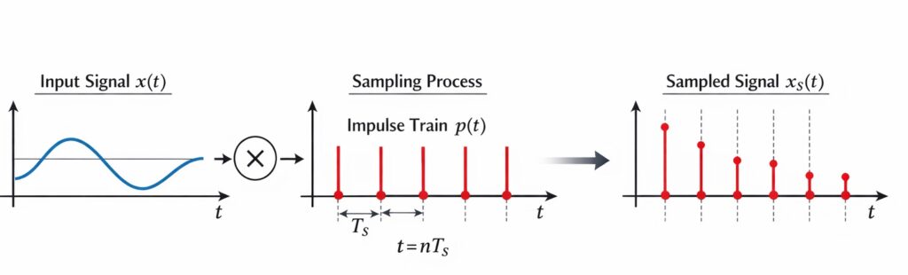
Principle of Ideal Sampling
In ideal sampling, the input signal is multiplied by an impulse train.
The impulse train is represented as
\[
p(t) = \sum_{n=-\infty}^{\infty} \delta(t-nT_s)
\]
where
\(\delta(t)\) = Dirac delta function
\(T_s\) = sampling period
The sampled signal becomes
\[
x_s(t) = x(t)\sum_{n=-\infty}^{\infty}\delta(t-nT_s)
\]
This produces impulses at time instants \(nT_s\) with amplitudes equal to
\(x(nT_s)\).
Characteristics of Ideal Sampling
Important characteristics include:
• Sampling occurs at exact time instants
• Each sample is represented by a Dirac impulse
• Pulse width is zero
• Sample amplitude equals the instantaneous value of the signal
• Used mainly for theoretical analysis
Frequency Domain Representation
In the frequency domain, ideal sampling produces periodic replicas of the original spectrum.
If \(X(f)\) is the spectrum of the signal, the sampled signal spectrum becomes
\[
X_s(f) = \frac{1}{T_s}\sum_{n=-\infty}^{\infty} X(f-nf_s)
\]
Thus, the original spectrum is repeated at multiples of the sampling frequency.
Aliasing
If the sampling frequency is less than the Nyquist rate, the spectral replicas overlap, producing aliasing distortion.
Aliasing causes loss of information, and the original signal cannot be recovered.
Ideal Sampling vs Natural Sampling vs Flat-Top Sampling
| Feature | Ideal Sampling | Natural Sampling | Flat-Top Sampling |
|---|---|---|---|
| Pulse width | Zero | Finite | Finite |
| Pulse shape | Impulse | Follows signal | Flat top |
| Practicality | Theoretical | Limited use | Widely used |
| Distortion | None | Very small | Aperture distortion |
Applications
Ideal sampling is used in:
• Sampling theorem analysis
• Digital signal processing theory
• Communication system design
• Signal reconstruction studies