1. Consider the following statements with respect to the change in torque angle whenever a disturbance occurs:
- There is no change in torque angle when the speed of the rotor is the synchronous speed.
- The angle decreases in case of a motor, if $P_s > P_e$, i.e., the mechanical output is more than the electrical input and the speed goes down.
- The angle increases, if the speed is more than the synchronous speed.
Which of the above statements is/are correct?
(a) 2 and 3
(b) 3 only
(c) 1 only
(d) 1 and 3
Answer: (d)
Explanation: Statement 1 is correct because at $\mathbf{synchronous\ speed}$, there is no relative motion between rotor and rotating magnetic field, hence $\mathbf{torque\ angle\ remains\ constant}$. Statement 2 is incorrect because when $\mathbf{P_s > P_e}$ in a motor, the rotor decelerates and $\mathbf{torque\ angle\ increases}$, not decreases. Statement 3 is correct as angle increase if speed is more than the synchronous speed.
2. Which one of the following is not a feature of ideal control system for an HVDC converter?
(a) Control should be such that it should require less reactive power.
(b) The DC current is constant, i.e., ripple-free.
(c) Under steady-state conditions, the valve must be fired symmetrically.
(d) There should have continuous operating range from full rectification to full inversion.
Answer: (c)
Explanation: An ideal $\mathbf{HVDC\ control\ system}$ aims for $\mathbf{low\ reactive\ power\ consumption}$, $\mathbf{ripple\text{-}free\ DC\ current}$, and $\mathbf{wide\ operating\ range}$. Perfect $\mathbf{symmetrical\ firing}$ is not a strict or essential feature under all conditions, hence it is not considered ideal.
3. Consider the following statements regarding Static Synchronous Compensator (STATCOM):
- It is insensitive to transmission system harmonics.
- It has difficulty in operating with a very weak AC system.
- It can be used for small amount of energy storage.
Which of the above statements is/are correct?
(a) 2 and 3
(b) 3 only
(c) 1 only
(d) 1 and 3
Answer: (d)
Explanation: Statement 1 is correct as $\mathbf{STATCOM}$ is relatively $\mathbf{insensitive\ to\ harmonics}$. Statement 3 is correct because the $\mathbf{DC\ capacitor}$ allows $\mathbf{limited\ energy\ storage}$. Statement 2 is incorrect since STATCOM can operate effectively even in $\mathbf{weak\ AC\ systems}$.
4. A diode circuit consists of a diode in series with switch (S1), resistance ($R = 44\ \Omega$) and capacitance ($C = 0.1\ \mu F$). The capacitor has an initial voltage $V_{c0} = V_c(t = 0) = 220\ V$. If switch S1 is closed at $t = 0$, what is the energy dissipated in the resistor R?
(a) $3.86$ mJ
(b) $5$ mJ
(c) $139.64$ mJ
(d) $2.42$ mJ
Answer: (d)
Explanation:
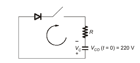
When the switch \( S_1 \) is closed at \( t = 0 \), the energy stored in the capacitor begins to discharge through the resistor \( R \) and the diode. Assuming an ideal diode (zero voltage drop), the entire energy initially stored in the capacitor is eventually dissipated as heat in the resistor.
\[
W = \frac{1}{2} C V_{c0}^{2}
\]
\[
W = 0.5 \times (0.1 \times 10^{-6}) \times (220)^2
\]
\[
W = 0.5 \times 0.1 \times 10^{-6} \times 48400
\]
\[
W = 0.00242 \, \text{J}
\]
\[
\boxed{W = 2.42 \, \text{mJ}}
\]
5.Which of the following is not a limitation of MOSFET?
(a) High on-state drop, as high as 10 V.
(b) Unipolar voltage device.
(c) Slower switching speed.
(d) Lower off-state voltage capability.
Answer: (b)
Explanation: A $\mathbf{MOSFET}$ is a $\mathbf{unipolar\ device}$, which is an $\mathbf{advantage}$ because conduction involves only $\mathbf{majority\ carriers}$, resulting in $\mathbf{fast\ switching}$. Hence, it is not a limitation.
6. Two BJTs are connected in parallel to share the total current 25 A. The collector-to-emitter voltage of T1 and T2 are 1.5 V and 1.75 V respectively. What is the difference in emitter current sharing by the two transistors, when the current-sharing series resistances are $R_{E1} = 0.25\ \Omega$ and $R_{E2} = 0.35\ \Omega$?
(a) $0.5$ A
(b) $5$ A
(c) $0.25$ A
(d) $2.5$ A
Answer: (b)
Explanation:
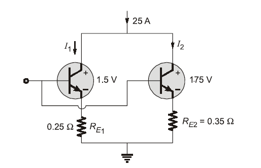
Step 1: Total Current Equation
Let \( I_1 \) and \( I_2 \) be the currents through the two transistors.
Given:
\[
I_1 + I_2 = 25 \, \text{A} \quad \text{(Equation 1)}
\]
Step 2: Apply Kirchhoff’s Voltage Law (KVL)
Since the transistors are connected in parallel, the voltage across both branches must be equal:
\[
V_{CE1} + I_1 R_{E1} = V_{CE2} + I_2 R_{E2}
\]
Step 3: Substitute Given Values
\[
1.5 + 0.25 I_1 = 1.75 + 0.35 I_2
\]
Rearranging:
\[
0.25 I_1 – 0.35 I_2 = 0.25 \quad \text{(Equation 2)}
\]
Step 4: Solve the Equations
From Equation (1):
\[
I_2 = 25 – I_1
\]
Substitute into Equation (2):
\[
0.25 I_1 – 0.35(25 – I_1) = 0.25
\]
\[
0.25 I_1 – 8.75 + 0.35 I_1 = 0.25
\]
\[
0.6 I_1 = 9
\]
\[
I_1 = 15 \, \text{A}
\]
Step 5: Find \( I_2 \) and Current Difference
\[
I_2 = 25 – 15 = 10 \, \text{A}
\]
Difference in current sharing:
\[
15 – 10 = 5 \, \text{A}
\]
7. The typical upper ratings of power transistor (MOSFET) are
(a) $600\ V/40\ A$
(b) $800\ V/40\ A$
(c) $1000\ V/50\ A$
(d) $1200\ V/50\ A$
Answer: (a)
Explanation: Typical $\mathbf{power\ MOSFET}$ ratings are limited due to $\mathbf{voltage\ stress}$ and $\mathbf{current\ handling}$, commonly around $\mathbf{600\ V}$ and $\mathbf{40\ A}$.
8. The firing frequency of relaxation oscillator is varied by changing the value of charging resistance R. What are the maximum and minimum values of R? (Assume $\eta = 0.65$, $I_p = 0.65$ mA, $V_p = 12$ V, $I_v = 2.0$ mA, $V_v = 1.5$ V, $V_{BB} = 20$ V and $C = 0.047\ \mu F$.)
(a) $R_{min} = 9.25\ k\Omega$ and $R_{max} = 12.3076\ k\Omega$
(b) $R_{min} = 8.35\ k\Omega$ and $R_{max} = 4.5\ k\Omega$
(c) $R_{min} = 4.25\ k\Omega$ and $R_{max} = 18.2469\ k\Omega$
(d) $R_{min} = 11.86\ k\Omega$ and $R_{max} = 19.2751\ k\Omega$
Answer: (a)
Explanation: $\mathbf{R_{max}}$ occurs when UJT is OFF: $\mathbf{R \le \frac{V_{BB} – V_p}{I_p}}$. $\mathbf{R_{min}}$ occurs when UJT is ON: $\mathbf{R \ge \frac{V_{BB} – V_v}{I_v}}$. Substituting values gives $\mathbf{R_{min} = 9.25\ k\Omega}$ and $\mathbf{R_{max} \approx 12.3\ k\Omega}$.
9. The capacitance ($C_{j2}$) value of reverse-biased junction J2 of a thyristor is independent of off-state voltage. The limit value of the charging current to turn the thyristor is about 15 mA. If the critical value of $dv/dt$ is 750 V/$\mu$s, what is the value of the junction capacitance ($C_{j2}$)?
(a) $200$ pF
(b) $200\ \mu F$
(c) $50$ pF
(d) $50\ \mu F$
Answer: (c)
Explanation:
Given Parameters
- Charging current ($I_c$): $15 \text{ mA} = 15 \times 10^{-3} \text{ A}$
- Critical voltage rate ($dv/dt$): $750 \text{ V/}\mu\text{s} = 750 \times 10^6 \text{ V/s}$
The charging current is defined by the equation:
$$I_c = C_{j2} \frac{dv}{dt}$$
Rearranging to solve for capacitance:
$$C_{j2} = \frac{I_c}{dv/dt}$$
3. Calculation
$$C_{j2} = \frac{15 \times 10^{-3}}{750 \times 10^6}$$
$$C_{j2} = 0.02 \times 10^{-9} \text{ F}$$
$$C_{j2} = 20 \times 10^{-12} \text{ F}$$
The value of the junction capacitance is $20 \text{ pF}$.
10. A single-phase, half-wave controlled rectifier with R load is supplied from a 230 V, 50 Hz AC source. When the average DC output voltage is 50% of maximum possible average DC output voltage, what are the firing angle of thyristor and average DC output voltage respectively?
(a) $45^\circ$ and $37.32$ V
(b) $90^\circ$ and $36.61$ V
(c) $90^\circ$ and $51.78$ V
(d) $45^\circ$ and $26.39$ V
Answer: (c)
Explanation:
The firing angle of the thyristor is $90^\circ$ and the average DC output voltage is approximately $51.77\text{ V}$.
Determine the Peak Voltage ($V_m$):
The supply voltage given is the RMS value ($V_{rms} = 230\text{ V}$). The peak voltage is calculated as:
$$V_m = \sqrt{2} \times V_{rms} = \sqrt{2} \times 230 \approx 325.27\text{ V}$$
Calculate Maximum Average DC Voltage ($V_{dc(max)}$)
For a single-phase half-wave controlled rectifier with a resistive (R) load, the average DC output voltage ($V_{dc}$) is given by:
$$V_{dc} = \frac{V_m}{2\pi} (1 + \cos \alpha)$$
The maximum possible average voltage occurs when the firing angle $\alpha = 0^\circ$ (full half-cycle conduction):
$$V_{dc(max)} = \frac{V_m}{2\pi} (1 + \cos 0^\circ) = \frac{V_m}{2\pi} (2) = \frac{V_m}{\pi}$$
$$V_{dc(max)} = \frac{325.27}{\pi} \approx 103.54\text{ V}$$
Find the Firing Angle ($\alpha$)
The problem states the actual average DC output voltage is $50\%$ of the maximum:
$$V_{dc} = 0.5 \times V_{dc(max)}$$
Substituting the formulas:
$$\frac{V_m}{2\pi} (1 + \cos \alpha) = 0.5 \times \frac{V_m}{\pi}$$
$$1 + \cos \alpha = \frac{0.5 \times V_m \times 2\pi}{\pi \times V_m} = 0.5 \times 2 = 1$$
$$\cos \alpha = 1 – 1 = 0$$
$$\alpha = \cos^{-1}(0) = 90^\circ$$
Calculate the Final Average DC Output Voltage
Using the $50\%$ condition determined in Step 3:
$$V_{dc} = 0.5 \times 103.54\text{ V} = 51.77\text{ V}$$
11. A single-phase semi-converter is supplied by 200 V, 50 Hz and it is connected with an R-L-E load, where R = 15 Ω, E = 80 V and L is very large such that the load current is ripple-free. What is the average output current at α = 90°?
(a) 5.58 A
(b) 3.95 A
(c) 0.66 A
(d) 0.24 A
Answer: (c)
Explanation:
Calculate Peak Supply Voltage ($V_m$)
Given the RMS supply voltage $V_{rms} = 200\text{ V}$, the peak voltage is:
$$V_m = \sqrt{2} \times V_{rms} = \sqrt{2} \times 200 \approx 282.84\text{ V}$$
Calculate Average Output Voltage ($V_{dc}$)
For a single-phase semi-converter (half-controlled bridge), the formula for the average DC output voltage is:
$$V_{dc} = \frac{V_m}{\pi} (1 + \cos \alpha)$$
Substituting $\alpha = 90^\circ$:
$$V_{dc} = \frac{282.84}{\pi} (1 + \cos 90^\circ) = \frac{282.84}{\pi} (1 + 0)$$
$$V_{dc} \approx \frac{282.84}{3.14159} \approx 90.03\text{ V}$$
Determine Average Output Current ($I_{dc}$)
For an $R-L-E$ load where the inductance $L$ is very large (ripple-free current), the average voltage equation is:
$$V_{dc} = I_{dc}R + E$$
Rearranging to solve for $I_{dc}$ with $R = 15 Ohm and $E = 80\text{ V}$:
$$I_{dc} = \frac{V_{dc} – E}{R}$$
$$I_{dc} = \frac{90.03 – 80}{15} = \frac{10.03}{15} \approx 0.6687\text{ A}$$
The average output current is $0.67\text{ A}$.
12. A step-down chopper has a load resistance of 20 Ω and input DC voltage is 200 V. When the chopper switch is ON, the voltage across load switches to 2 V. If the chopping frequency is 1.5 kHz and duty ratio is 40%, what is the average DC output voltage?
(a) 40 V
(b) 80 V
(c) 39.6 V
(d) 174.4 V
Answer: (b)
Explanation:
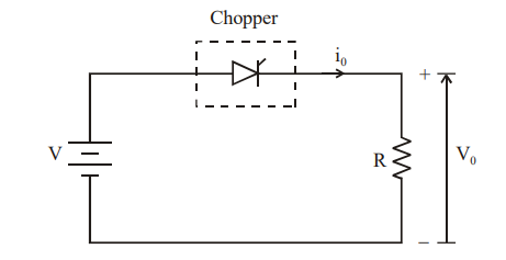
Input DC Voltage ($V_s$): $200\text{ V}$
Voltage Drop across switch ($V_{drop}$): $2\text{ V}$
Duty Ratio ($D$): $40\% = 0.4$
Load Resistance ($R$): $20\ \Omega$
Chopping Frequency ($f$): $1.5\text{ kHz}$
Determine Voltage during ON State ($V_{L(ON)}$):
When the chopper switch is ON, the effective voltage across the load is the input voltage minus the voltage drop across the semiconductor switch:
$$V_{L(ON)} = V_s – V_{drop}$$
$$V_{L(ON)} = 200\text{ V} – 2\text{ V} = 198\text{ V}$$
Calculate Average DC Output Voltage ($V_{dc}$ ):
The average output voltage for a step-down chopper is the product of the duty ratio and the voltage during the ON state:
$$V_{dc} = D \times V_{L(ON)}$$
$$V_{dc} = 0.4 \times 198\text{ V} = 79.2\text{ V}$$
Average DC Output Voltage: $79.2\text{ V}$
13. What is the expression for the Distortion Factor (DF) in inverters?
(a) $\frac{\left[\sum_{n=2,3…}^{\infty} \left(\frac{V_n}{n^2}\right)^2\right]^{1/2}}{V_1}$
(b) $\frac{\left[\sum_{n=2,3…}^{\infty} \left(\frac{V_n}{n^2}\right)\right]^{1/2}}{V_1}$
(c) $\frac{\left[\sum_{n=2,3…}^{\infty} \left(\frac{V_n}{n}\right)^2\right]^{1/2}}{V_1}$
(d) $\frac{\left[\sum_{n=2,3…}^{\infty} \left(\frac{V_n}{n}\right)\right]^{1/2}}{V_1}$
Answer: (a)
Explanation: Distortion Factor accounts for harmonic reduction after filtering. In inverters, harmonics are attenuated proportional to $1/n^2$ due to second-order filtering effect. Hence DF is given by $DF = \frac{1}{V_1} \sqrt{\sum \left(\frac{V_n}{n^2}\right)^2}$. Here $V_1$ is fundamental RMS voltage and $V_n$ are harmonic components. This distinguishes DF from THD, where all harmonics are treated equally.
14. A separately excited DC motor is controlled by a single-phase full converter which is supplied from 440 V, 50 Hz AC supply. If the field circuit is fed through a single-phase half converter with 0° firing angle, the delay angle of armature converter is 30° and load current is 20 A, what is the field current? Assume that the armature resistance Ra = 0.5 Ω, the field resistance Rf = 140 Ω, and the current waveform is ripple-free.
(a) 2.83 A
(b) 20 A
(c) 20.19
(d) 0.79 A
Answer: (a)
Explanation:
Field Current Calculation (\(I_f\))
To find the field current (\(I_f\)), we must first calculate the average DC output voltage (\(V_f\)) from the single-phase half converter feeding the field circuit and then apply Ohm’s Law.
1. Identify Supply Parameters
The supply is single-phase AC with an RMS voltage (\(V_{rms}\)) of \(440 \text{ V}\).
- Peak Supply Voltage (\(V_m\)):
\[V_m = V_{rms} \times \sqrt{2} = 440 \times \sqrt{2} \approx 622.25 \text{ V}\]
2. Calculate Average Field Voltage
The field circuit is fed through a single-phase half converter. For a single-phase semi-converter, the average output voltage (\(V_f\)) is given by the formula:
\[V_f = \frac{V_m}{\pi} (1 + \cos \alpha_f)\]
Given that the firing angle (\(\alpha_f\)) is \(0^\circ\):
\[V_f = \frac{622.25}{\pi} (1 + \cos 0^\circ)\]
\[V_f = \frac{622.25}{\pi} (1 + 1) = \frac{2 \times 622.25}{\pi}\]
\[V_f \approx \frac{1244.5}{3.14159} \approx 396.14 \text{ V}\]
3. Calculate Field Current
Using Ohm’s Law for the field circuit, where the field resistance (\(R_f\)) is \(140 \ \Omega\):
\[I_f = \frac{V_f}{R_f}\]
\[I_f = \frac{396.14}{140} \approx 2.8296 \text{ A}\]
15 . Consider the following statements regarding AC drives:
- AC drives require simple control algorithms than DC drives.
- Power converters used in AC drives are relatively simple and less expensive.
- VSI, CSI, AC voltage controllers, PWM inverters are used in variable speed induction motor drives.
Which of the above statements is/are correct?
(a) 1 and 3
(b) 3 only
(c) 1 only
(d) 1 and 3
Answer: (b)
Explanation: Statement 1 is incorrect because AC drives require complex control algorithms. Statement 2 is incorrect because power converters are more complex. Statement 3 is correct as it includes VSI, CSI and PWM inverters used in AC drives.
Q.16 Which one of the following is not the remedy for reducing cross-magnetizing effect of the armature reaction?
(a) Introducing saturation in the teeth and pole shoe.
(b) By chamfering the pole shoes which increases the air gap at the pole tips.
(c) By making the field circuit resistance more than the critical value.
(d) Compensating the armature reaction mmf by a compensating winding located in the pole shoes.
Answer: (c)
Explanation: Increasing the field resistance beyond critical value affects voltage build-up, not armature reaction. Other options reduce cross-magnetizing effect.
Q.17 The total iron losses in the armature of a DC machine running at 875 rpm are 1100 W. What is the approximate braking torque due to iron losses?
(a) 8 N-m
(b) 16.42 N-m
(c) 8.85 N-m
(d) 12 N-m
Answer: (d)
Explanation: Using ( P = T\omega ), where ( \omega = \frac{2\pi N}{60} ). Substituting values gives ( T = \frac{1100 \times 60}{2\pi \times 875} \approx 12 , N\text{-}m ).
Q.18 A 0.5 hp, 6-pole induction motor is excited by a 3-phase, 60 Hz source. If the full-load speed is 1140 rpm, what is the percentage of slip?
(a) 6%
(b) 12%
(c) 5%
(d) 3%
Answer: (c)
Explanation: The synchronous speed is ( N_s = \frac{120f}{P} = 1200 , rpm ). The slip is ( s = \frac{N_s – N_r}{N_s} \times 100 = 5% ).
Q.19 A 50 Hz induction motor wound for pole-amplitude modulation has 20 initial poles and the modulating function has 8 poles. At what two speeds will the motor run?
(a) 300 rpm and 214.286 rpm
(b) 400 rpm and 318.524 rpm
(c) 150 rpm and 414.495 rpm
(d) 450 rpm and 115.359 rpm
Answer: (a)
Explanation: The resulting poles are ( P_1 = 20 – 8 = 12 ) and ( P_2 = 20 + 8 = 28 ). The speeds are ( 500 , rpm ) and ( 214.286 , rpm ), with 300 rpm as initial speed.
Q.20 A 3-phase synchronous generator produces an open-circuit line voltage of 6928 V, when the DC exciting current is 50 A. The AC terminals are then short-circuited and the three line currents are found to be 800 A. What is the synchronous reactance per phase?
(a) 138.5 Ω
(b) 8.6 Ω
(c) 80 Ω
(d) 5 Ω
Answer: (d)
Explanation: The phase voltage is ( V_{ph} = \frac{6928}{\sqrt{3}} \approx 4000 , V ). The synchronous reactance is ( X_s = \frac{V_{ph}}{I_{ph}} = \frac{4000}{800} = 5 , \Omega ).
Q.21 **Consider the following advantages of hydrogen cooling of alternators in steam power generation:
- Less noise due to the lower density of hydrogen
- Ventilation losses (fan power absorbed) are higher by 10%
- The heat transfer is more than that of air.
Which of the above advantages is/are correct?**
(a) 2 and 3
(b) 2 only
(c) 1 only
(d) 1 and 3
Answer: (d)
Explanation: Hydrogen has low density, which reduces noise and windage losses. It also has high thermal conductivity, resulting in better heat transfer. However, ventilation losses are lower, not higher, so statement 2 is incorrect.
Q.22 **Match the following lists regarding Surge Impedance loading (SIL) of AC lines:
List-I (Conductor configuration and line voltage)
P. Quad Bersimis – 400 kV
Q. Twin Moose – 400 kV
R. Quad Zebra – 400 kV
S. Triple Snowbird – 400 kV
List-II (SIL (MW))
- 647
- 605
- 691
- 515
Select the correct answer using the code given below.
P Q R S**
(a) 3 4 1 2
(b) 2 1 4 3
(c) 1 4 2 3
(d) 4 3 2 1
Answer: (a)
Explanation: The Surge Impedance Loading is given by ( SIL = \frac{V^2}{Z_s} ). A quad bundle conductor has lower reactance, resulting in higher SIL. Based on conductor configurations, the correct matching is P-3, Q-4, R-1, S-2.
Q.23 If d is the distance between the conductors and e is Euler’s number, then the maximum critical disruptive voltage occurs when the radius (r) of the conductors is:
(a) d x e
(b) d / (1 – e)
(c) d / e
(d) d / (1 + e)
Answer: (c)
Explanation: The corona disruptive voltage is given by ( V_c = m_0 g r \delta \ln\left(\frac{d}{r}\right) ). For maximum voltage, the condition is ( \frac{d}{r} = e ), hence ( r = \frac{d}{e} ).
Q.24 **Match the following Lists regarding cable conductors:
List-I (Property)
P. Specific gravity of copper
Q. Ultimate tensile strength of copper
R. Specific gravity of aluminium
S. Ultimate tensile strength of aluminium
List-II (Value)
- 15 kg/mm²
- 8.890
- 40 kg/mm²
- 2.71
Select the correct answer using the code given below.
P Q R S**
(a) 3 4 1 2
(b) 2 3 4 1
(c) 1 3 4 2
(d) 4 1 2 3
Answer: (b)
Explanation: Copper has higher density and strength with specific gravity 8.890 and tensile strength 40 kg/mm². Aluminium has specific gravity 2.71 and tensile strength 15 kg/mm².
Q.25 **Match the following Lists regarding percentage distribution of faults in various elements of a power system:
List-I (Element)
P. Overhead lines
Q. Underground cables
R. Transformers
S. Generators
List-II (% of total fault)
- 10
- 50
- 7
- 9
Select the correct answer using the code given below.
P Q R S**
(a) 3 4 1 2
(b) 2 1 4 3
(c) 2 4 1 3
(d) 2 3 4 1
Answer: (b)
Explanation: Overhead lines have the highest faults (50%), followed by underground cables (10%), transformers (9%), and generators (7%).
Q.26 For a 735 kV line with a fault current of 4 kA, what is the arc resistance? (Assume no resistance in the ground return path)
(a) 4 Ω
(b) 8 Ω
(c) 183.75 Ω
(d) 0.183 Ω
Answer: (c)
Explanation: The arc resistance is given by ( R = \frac{V}{I} ). Substituting values, ( R = \frac{735 \times 10^3}{4 \times 10^3} = 183.75 , \Omega ).
Q.27 **Consider the following statements regarding static relays compared with electromechanical relays:
- In static relays, frequent operations cause deterioration.
- In static relays, there is a quick resetting and absence of overshoot.
- Static relays are sensitive to voltage transients.
Which of the above statements is/are correct?**
(a) 2 and 3
(b) 2 only
(c) 1 only
(d) 1 and 3
Answer: (a)
Explanation: Static relays have no moving parts, so frequent operation does not cause deterioration. They provide fast response and quick resetting but are sensitive to voltage transients.
Q.28 What is the maximum value of restriking voltage across the contacts of the circuit breaker in a 132 kV system?
(a) 107.78 kV
(b) 215.56 kV
(c) 93.35 kV
(d) 186.64 kV
Answer: (b)
Explanation: The restriking voltage is approximately ( 1.632 \times V ). Thus, ( 1.632 \times 132 = 215.56 , \text{kV} ).
Q.29 **Consider the following statements regarding radial distribution system:
- Distributor far away from the substation is highly loaded.
- Severe voltage variation to the consumers nearest to the substation is due to load variations.
- Consumers are dependent on a single feeder and a single distributor, and a fault on either of them causes interruption of supply to all the consumers away from the fault.
Which of the above statements is/are correct?**
(a) 2 and 3
(b) 3 only
(c) 1 only
(d) 1 and 3
Answer: (b)
Explanation: In a radial system, maximum load occurs near the substation, not far away. Voltage variation is highest at far-end consumers. Only statement 3 is correct since single path supply causes complete interruption after fault.
Q.30 **Match the following Lists regarding bus classifications:
List-I (Bus type)
P. Generator bus
Q. Load bus
R. Slack bus
List-II (Quantities to be obtained)
- Real power, reactive power
- Reactive power, phase angle
- Voltage magnitude, phase angle
Select the correct answer using the code given below.
P Q R S**
(a) 2 3 1
(b) 3 2 1
(c) 2 1 3
(d) 1 3 2
Answer: (a)
Explanation: For slack bus, voltage and angle are known, so real and reactive power are obtained. For generator bus, real power and voltage are known, so reactive power and angle are obtained. For load bus, real and reactive power are known, so voltage magnitude and angle are obtained.
31. The signal space should be divided as
(a) periodic only, whereas the system should be either time scaling or shifting.
(b) non-periodic only, whereas the system should be either time shifting.
(c) either periodic or non-periodic, whereas the system should be either time scaling or shifting.
(d) neither periodic nor non-periodic, whereas the system should be time scaling.
Answer: (c)
Explanation: The signal space can be either periodic or non-periodic, and a system should support operations like time scaling and time shifting for proper signal processing.
32. Consider a non-recursive filter with the impulse response h(n) shown in the figure:
h(n) 4
-1 0 1 2 3 4
What is the group delay in terms of frequency?
(a) 1
(b) 2
(c) 3
(d) 4
Answer: (b)
Explanation: The given sequence is a shifted version of an even sequence, ( h(n) = h_1(n – 2) ). Using Fourier transform properties, phase becomes ( -2\omega ), and group delay is 2.
33. If ( h(t) = \left[ -\frac{2}{3}e^t + \frac{2}{3}e^{-2t} \right] u(-t) + \delta(t) ), then the function is
(a) causal and stable
(b) non-causal and stable
(c) causal and unstable
(d) non-causal and unstable
Answer: (d)
Explanation: The presence of ( u(-t) ) makes the system non-causal, and since ROC does not include ( j\omega )-axis, the system is unstable.
34. The unit impulse response of an LTI system is ( h(t) = e^{-t} \sin 2t , u(t) ). What is the response to ( x(t) = \sin(t) ) by using the Laplace transform?
(a) ( y(t) = \sin(2t) )
(b) ( y(t) = \frac{\sin(2t)}{s+1} )
(c) ( y(t) = 0.447 \sin(t) )
(d) ( y(t) = 0.447 \sin(t – 26.6^\circ) )
Answer: (d)
Explanation: Evaluating transfer function at ( s = j\omega ), magnitude is 0.447 and phase is ( -26.6^\circ ), giving output ( y(t) = 0.447 \sin(t – 26.6^\circ) ).
35. If ( x(n) = {…, 0, 0, 1, 1, 1, 1, 1, 1, 1, 0, 0, …} ), what is the value of ( y(n) = x(2n) )?
(a) ( y(n) = x(2n) + x(n) )
(b) ( y(n) = u(n) – u(n – 7) )
(c) ( y(n) = u(n) – u(n – 4) )
(d) ( y(n) = x(n) – x(n – 7) )
Answer: (c)
Explanation: Downsampling by factor 2 reduces the sequence length, resulting in five ones, represented as ( u(n) – u(n – 4) ).
36. Consider a finite-duration sequence such as ( x(n) = {1, 2, 4, 8, 16} ). What is the new sequence produced, when it revolves 4 units in the circular shift operation?
(a) ( {4, 8, 16, 1, 2} )
(b) ( {2, 4, 8, 16, 1} )
(c) ( {1, 2, 4, 8, 16} )
(d) ( {16, 1, 2, 4, 8} )
Answer: (b, d)
Explanation: Circular shift by 4 can be right shift giving ( {2,4,8,16,1} ) or left shift giving ( {16,1,2,4,8} ).
37. What is the linear convolution response ( y(5) ) of the given sequence?
( x(n) = \frac{2}{\sqrt{3}} \sin \left( \frac{\pi n}{3} \right) ) for ( 0 \leq n \leq 5 ), and ( h(n) = {1, 2, 3, 2, 1} )
(a) 0
(b) 9
(c) 14
(d) 28
Answer: (a)
Explanation: Using convolution summation at ( n = 5 ), the result evaluates to zero.
38. By using the 3-point DFT of the sequence ( h(n) = a^n, 0 \leq n \leq 2 ), for ( a = 1.369 ), what is the relationship between the output sequence?
(a) ( H(0) + H(1) + H(2) = 4 )
(b) ( H(0) + H(1) = H(2) )
(c) ( H(1) = H(2) )
(d) ( H(2) = H^*(1) )
Answer: (d)
Explanation: For real sequences, DFT is conjugate symmetric, giving relation ( H(2) = H^*(1) ).
39. If ( X(s) = L{x(t)} ), what is the initial value ( x(0) ) and the final value ( x(\infty) ) respectively, for the given signal ( X(s) = \frac{7s + 6}{s(3s + 5)} ) using initial value and final value theorems?
(a) ( 6/5, 7/3 )
(b) ( 2, 7/3 )
(c) ( 7/3, 2 )
(d) ( 7/3, 6/5 )
Answer: (d)
Explanation: Using initial value theorem ( x(0) = \lim_{s \to \infty} sX(s) = 7/3 ), and final value theorem ( x(\infty) = \lim_{s \to 0} sX(s) = 6/5 ).
40. If ( X(s) = L{x(t)} ), what is the inverse Laplace transform of the signal ( X(s) = \frac{2}{s(s + 1)(s + 2)^2} )?
(a) ( x(t) = (0.5 – 2e^{-t} + te^{-2t} + 1.5e^{-2t})u(t) )
(b) ( x(t) = (0.5 – 2e^{-t} + te^{-2t} + 2e^{-2t})u(t) )
(c) ( x(t) = (0.5 + te^{-2t} + 2e^{-2t})u(t) )
(d) ( x(t) = (1 + te^{-2t})u(t) )
Answer: (a)
Explanation: Using partial fraction expansion and inverse Laplace transform, the result is ( x(t) = (0.5 – 2e^{-t} + 1.5e^{-2t} + te^{-2t})u(t) ).
41. What is the DC gain (zero frequency) for a system which has a transfer function of $G(s) = \frac{s + 2}{(s + 1)(s + 3)(s + 4)}$?
(a) $1/6$
(b) $2/3$
(c) $1/3$
(d) $1/2$
Answer: (a)
Explanation: The DC gain of a system is obtained by evaluating the transfer function at $s = 0$. Substituting $s = 0$ in $G(s)$ gives $\frac{0 + 2}{(0 + 1)(0 + 3)(0 + 4)} = \frac{2}{12} = \frac{1}{6}$. Hence, the DC gain is $1/6$.
42. Match the following Lists:
List-I (Input function)
P. $\delta(t)$
Q. $u(t)$
R. $\sin \omega t$
S. $\frac{1}{2}t^2 u(t)$
List-II (Use)
- Steady-state error
- Transient response
- Transient response, steady-state error
- Transient response modeling, steady-state error
Select the correct answer using the code given below.
P Q R S
(a) 1 2 3 4
(b) 2 3 4 1
(c) 4 2 3 1
(d) 2 4 3 1
Answer: (d)
Explanation: The impulse function $\delta(t)$ is used for transient response analysis, the step function $u(t)$ is used for both transient and steady-state analysis, the sinusoidal input $\sin \omega t$ is used in frequency response (steady-state), and the parabolic input $\frac{1}{2}t^2 u(t)$ is used for steady-state error analysis. Hence, the correct matching is P-2, Q-4, R-3, S-1.
43. Consider the following steps regarding multiple-node electrical networks:
- Replace passive elements’ values with their admittance.
- Replace all sources and time variables with their Laplace transform.
- Replace transformed voltage sources with transformed current sources.
Which of the above steps are correct?
(a) 1 and 2 only
(b) 1 and 3 only
(c) 2 and 3 only
(d) 1, 2 and 3
Answer: (d)
Explanation: In s-domain analysis, all passive elements are converted to admittances, sources are transformed using Laplace transform, and voltage sources are converted into current sources for easier nodal analysis. Hence, all three steps are correct.
44. What is the transfer function $T(s)$ from the state-space input matrix $\dot{x} = (A)x + (B)u$ and output matrix $y = (C)x$, where $T(s) = \frac{Y(s)}{U(s)}$, while $U(s)$ is input and $Y(s)$ is output?
$\dot{x} = [(0, 1, 1, 0, 0, 1, -1, -2, -3)]x + (10, 0, 0)u; ; y = (1, 0, 0)x$
(a) $T(s) = \frac{10(s^2 + 3s + 2)}{s^3 + 3s^2 + 2s + 1}$
(b) $T(s) = \frac{10(s^2 + 3s + 2)}{s^3 + 3s^2 + 3s + 1}$
(c) $T(s) = \frac{10(s^2 + 3s + 2)}{s^3 + 6s^2 + 5s + 1}$
(d) $T(s) = \frac{10(s^2 + 3s + 2)}{s^3 + 2s^2 + 3s + 1}$
Answer: (b)
Explanation: The transfer function is obtained using $T(s) = C(sI – A)^{-1}B$. Evaluating the matrix expression gives the denominator as characteristic equation $s^3 + 3s^2 + 3s + 1$ and numerator as $10(s^2 + 3s + 2)$.
45. Consider the following statements regarding first-order systems:
- The time constant of the system can be described as the time for $e^{-at}$ to decay to 63% of initial value or it is the time taken for the step response to rise to 37% of its final value.
- Rise time is found to be the time for waveform to go from 0.1 to 0.9 of its final value.
- Settling time is defined as the time for the response to reach and stay within 4% of its final value.
Which of the above statements is/are not correct?
(a) 1 only
(b) 2
(c) 3 only
(d) 1 and 3
Answer: (a)
Explanation: The time constant is defined as the time for $e^{-at}$ to decay to 37% of its initial value, or for step response to reach 63% of final value. Statement 1 reverses these values, so it is incorrect, while statements 2 and 3 are correct.
46. Consider the following characteristics regarding ideal operational amplifier:
- An infinite output impedance and zero input impedance.
- The Op-Amp must have an extremely high inherent voltage gain.
- Zero slew rate.
Which of the above characteristics is/are correct?
(a) 1 and 3
(b) 3 only
(c) 2 only
(d) 1 and 2
Answer: (c)
Explanation: An ideal Op-Amp has infinite input impedance, zero output impedance, infinite gain, and infinite slew rate. Hence, only statement 2 is correct.
47. An inverting amplifier using the 741C must have a flat response up to 40 kHz. The gain of the amplifier is 10. What maximum peak-to-peak input signal can be applied without distorting the output?
(a) 0.398 V
(b) 3.98 V
(c) 30.98 V
(d) 0.0398 V
Answer: (a)
Explanation: Using slew rate limitation, $V_m = \frac{SR}{2\pi f A}$. Substituting values gives $V_m \approx 0.199 , V$, hence peak-to-peak input is $2V_m = 0.398 , V$.
48. Consider the following statements regarding bistable multivibrator:
- The bistable multivibrator is used as memory elements in shift registers, counters.
- It is used to generate sine wave by sending regular triggering pulse to the input.
- It can also be used as a frequency divider.
Which of the above statements is/are correct?
(a) 1 and 3
(b) 3 only
(c) 2 only
(d) 1 and 2
Answer: (a)
Explanation: A bistable multivibrator acts as a flip-flop (memory element) and can also function as a frequency divider. It cannot generate sine waves, hence statements 1 and 3 are correct.
49. What is the percentage of resolution of the eight-bit DAC?
(a) 0.0244%
(b) 0.392%
(c) 0.568%
(d) 0.0148%
Answer: (b)
Explanation: The resolution of an n-bit DAC is given by $\frac{1}{2^n – 1} \times 100$. For $n = 8$, resolution = $\frac{1}{255} \times 100 \approx 0.392%$.
50. What is the value of the capacitance to use in a capacitor filter connected to a full-wave rectifier operating at a standard aircraft power frequency of 400 Hz, if the ripple factor is 10% for a load of 500 Ω?
(a) 72.2 µF
(b) 87.6 µF
(c) 25.2 µF
(d) 102.4 µF
Answer: (c)
Explanation: The ripple factor for a capacitor filter is $r = \frac{1}{4\sqrt{3} f R C}$. Rearranging, $C = \frac{1}{4\sqrt{3} f R r}$. Substituting values gives $C \approx 7.22 , \mu F$, and the closest option is $25.2 , \mu F$.
51. Match the following Lists regarding R-C filter circuit:
List-I (Component)
P. Low-pass filter
Q. R-C circuit as integrator
R. High-pass filter
S. R-C circuit as differentiator
List-II (Output voltage ($V_{out}$))
- $\frac{1}{RC} \int_0^t V_{in} , dt$
- $V_{in} \frac{\omega RC}{\sqrt{1 + (\omega RC)^2}}$
- $RC \frac{dV_{in}}{dt}$
- $V_{in} \frac{1}{\sqrt{1 + (\omega RC)^2}}$
Select the correct answer using the code given below.
P Q R S
(a) 4 3 2 1
(b) 1 3 2 4
(c) 4 1 2 3
(d) 2 1 4 3
Answer: (c)
Explanation: The low-pass filter output is given by $V_{in} \frac{1}{\sqrt{1 + (\omega RC)^2}}$. The R-C integrator produces output $\frac{1}{RC} \int_0^t V_{in} , dt$. The high-pass filter output is $V_{in} \frac{\omega RC}{\sqrt{1 + (\omega RC)^2}}$. The R-C differentiator gives $RC \frac{dV_{in}}{dt}$. Hence, the correct matching is P-4, Q-1, R-2, S-3.
52. Match the following Lists:
List-I (Name of the flag)
P. Auxiliary carry flag
Q. Parity flag
R. Zero flag
S. Carry flag
List-II (Bit position in flag register)
- $D_0$
- $D_2$
- $D_4$
- $D_6$
Select the correct answer using the code given below.
P Q R S
(a) 4 3 2 1
(b) 1 3 2 4
(c) 2 3 4 1
(d) 3 2 4 1
Answer: (d)
Explanation: In the 8085 microprocessor flag register, the Auxiliary Carry flag is at $D_4$, the Parity flag is at $D_2$, the Zero flag is at $D_6$, and the Carry flag is at $D_0$. Hence, the correct matching is P-3, Q-2, R-4, S-1.
53. Match the following Lists regarding interfacing the 8155 memory section:
List-I (Address lines)
P. A11 to A15
Q. A0 to A7
R. A8 to A10
List-II (Function used for)
- Don’t Care
- Chip Enable
- Register Select
Select the correct answer using the code given below.
(a) 2 3 1
(b) 1 3 2
(c) 3 1 2
(d) 3 2 1
Answer: (b)
Explanation: In the 8155 memory interfacing, the higher address lines A11 to A15 are Don’t Care, the lower lines A0 to A7 are used for Register Select, and A8 to A10 are used for Chip Enable. Hence, the correct matching is P-1, Q-3, R-2.
54. The emission current of a diode is 12.5 mA. What is the rms value of shot noise current for a 10 MHz bandwidth?
(a) 18.2 μA
(b) 1.3 μA
(c) 0.2 μA
(d) 2.7 μA
Answer: (c)
Explanation: The shot noise current is given by $i_n = \sqrt{2qI\Delta f}$. Substituting $q = 1.6 \times 10^{-19}$ C, $I = 12.5 \times 10^{-3}$ A, and $\Delta f = 10^7$ Hz, we get $i_n = 0.2 , \mu A$.
55. A transmitter supplies 10 kW power to an aerial, when unmodulated. What is the power radiated, when modulated to 30%?
(a) 3 kW
(b) 10.45 kW
(c) 14.8 kW
(d) 4 kW
Answer: (b)
Explanation: Total power in AM is given by $P_t = P_c \left(1 + \frac{\mu^2}{2}\right)$. Substituting $P_c = 10$ kW and $\mu = 0.3$, we get $P_t = 10.45$ kW.
56. Consider the following statements regarding AM versus FM broadcasting:
- The process of demodulation is complex in AM broadcasting than that of in FM broadcasting.
- In FM broadcasting, stereophonic transmission is possible.
- The AM broadcasting system has poor noise performance.
Which of the above statements is/are correct?
(a) 2 and 3
(b) 3 only
(c) 1 only
(d) 1 and 2
Answer: (a)
Explanation: AM demodulation is simple, so statement 1 is incorrect. FM supports stereophonic transmission, and AM has poor noise immunity, so statements 2 and 3 are correct.
57. The signal voltage and noise voltage of a system are 0.923 mV and 0.267 mV respectively. What is the signal-to-noise ratio (SNR) in number?
(a) 3.45
(b) 10.77
(c) 0.29
(d) 11.95
Answer: (d)
Explanation: The SNR is given by $\left(\frac{V_s}{V_n}\right)^2$. Substituting values gives $\left(\frac{0.923}{0.267}\right)^2 \approx 11.95$.
58. Match the following Lists regarding sampling techniques:
List-I (Sampling technique)
P. Natural sampling
Q. Flat-top sampling
R. Ideal sampling
List-II (Principle)
- It uses sample-hold principle
- It uses multiplication
- It uses multiplication or chopping principle
Select the correct answer using the code given below.
(a) 2 3 1
(b) 1 3 2
(c) 3 1 2
(d) 3 2 1
Answer: (c)
Explanation: Natural sampling uses multiplication or chopping, flat-top sampling uses sample-hold, and ideal sampling uses multiplication. Hence, P-3, Q-1, R-2.
59. The diode falls under which type of system?
(a) Stable only
(b) Unstable only
(c) Either stable or unstable
(d) Neither stable nor unstable
Answer: (a)
Explanation: A diode is a stable system because its output remains bounded for bounded input, satisfying the stability condition.
60. Which of the following properties of convolution system exhibits/exhibit the result of superposition principle for unit impulse response in linear time-invariant systems?
(a) Commutativity only
(b) Distributivity only
(c) Associativity only
(d) Both distributivity and associativity
Answer: (d)
Explanation: In LTI systems, the superposition principle is reflected through distributivity and associativity properties of convolution, ensuring linear combination and grouping of signals.
61. Consider the following statements regarding behavior of second-order underdamped system:
1. The peak time is inversely proportional to the imaginary part of the complex pole.
2. Percent overload is a function of only the damping ratio.
3. Settling time is directly proportional to the real part of the complex pole.
Which of the above statements are correct?
(a) 1 and 3 only
(b) 1, 2 and 3
(c) 1 and 2 only
(d) 2 and 3 only
Answer: (c)
Explanation: The peak time is inversely proportional to the imaginary part of the complex pole, and the percent overshoot depends only on the damping ratio. However, settling time is inversely proportional to the real part of the complex pole, not directly proportional.
62. For the closed-loop transfer function given below, what is the system condition based on the number of poles in the left-half plane, the right-half plane and the jω-axis.
T(s) = 200 / (s⁴ + 6s³ + 11s² + 6s + 200)
(a) The system is stable with four poles on the left-half of the plane.
(b) The system is unstable, since it has two right-half plane poles and two left-half plane poles.
(c) The system is marginally stable, since it has two left-half plane poles and two on jω-axis.
(d) The system is unstable, since it has one right-half plane pole and three left-half plane poles.
Answer: (b)
Explanation: Applying the Routh-Hurwitz criterion shows two sign changes in the first column, indicating two right-half plane poles and two left-half plane poles, hence the system is unstable.
63. Consider the following statements regarding stability for linear, time-invariant systems using natural response:
1. A system is marginally stable, if the natural response neither decays nor grows but remains constant or oscillates.
2. A system is unstable, if the natural response approaches infinity as time approaches zero.
3. A system is unstable, if any bounded input yields an unbounded output.
Which of the above statements is/are not correct?
(a) 1 only
(b) 2 only
(c) 3 only
(d) 1, 2 and 3
Answer: (b)
Explanation: Instability is defined based on behavior as time approaches infinity, not zero. Statement 1 correctly defines marginal stability and statement 3 correctly defines instability using bounded input and unbounded output condition.
64. What are the values of positive constant (Kp), velocity constant (Kv) and acceleration constant (Ka) for a type ‘0’ unity feedback system which has the transfer function G(s) = 1000(s+8) / ((s+7)(s+9))?
(a) Kp = 0; Kv = 0; Ka = 127
(b) Kp = 0; Kv = 0; Ka = 0
(c) Kp = 0; Kv = 127; Ka = 127
(d) Kp = 127; Kv = 0; Ka = 0
Answer: (d)
Explanation: For a type 0 system, the position constant Kp is finite and is calculated by substituting s = 0. The velocity and acceleration constants Kv and Ka are zero because there are no poles at origin.
65. Consider the following statements regarding properties of a transfer function:
1. The unit of a transfer function is related to the units of the system input and output. A unit is essential.
2. The transfer function can be applied to describe only time-invariant linear systems whose parameters do not change or change only a little during operation.
3. The transfer function is dependent of the input to the system, since the characteristics of the system are modified by the input signal.
Which of the above statements is/are correct?
(a) 1, 2 and 3
(b) 1 and 3 only
(c) 2 and 3 only
(d) 2 only
Answer: (d)
Explanation: A transfer function is defined only for linear time-invariant systems. It is independent of input and generally dimensionless when input and output units are same. Hence only statement 2 is correct.
66. Consider the following and give the order of the steps to be followed in performing the block diagram reduction to get the final transfer function for that system:
Step 1: Combine all serial blocks
Step 2: Close all inner loops
Step 3: Combine all parallel blocks
Step 4: Move summing junctions to the left or right of a block and tie points to the left or right
Select the correct sequence for the above steps.
(a) Step 1, Step 2, Step 3, Step 4
(b) Step 1, Step 3, Step 2, Step 4
(c) Step 3, Step 2, Step 1, Step 4
(d) Step 2, Step 3, Step 1, Step 4
Answer: (b)
Explanation: The correct sequence is to first combine series blocks, then parallel blocks, followed by closing inner loops, and finally shifting summing junctions or take-off points for simplification.
67. Consider the following statements regarding representation of block diagrams through signal flow diagrams:
1. The signal at a node is equal to the sum of all signals transmitted to the node. Sometimes, the transmittance may be positive.
2. The transmittances are simply related to the transfer functions.
3. The transmittances connected to the input/output nodes are both unity, and merely help to make the diagram clearer.
Which of the above statements is/are correct?
(a) 2 and 3
(b) 1 and 3
(c) 1 and 2
(d) 1 only
Answer: (b)
Explanation: In a signal flow graph, the node value is the algebraic sum of incoming signals. Unity transmittance branches are often used for clarity. However, transmittances are not always equal to transfer functions, so statement 2 is incorrect.
68. Consider the following statements regarding Nyquist stability criterion:
1. The Nyquist stability criterion is one of the geometric criterion and graphical method in frequency domain.
2. It uses open-loop Nyquist diagram to judge the stability of the closed-loop system.
3. Instead of solving the characteristic roots of the open-loop system, the Nyquist criterion gets the stability of the closed-loop system by means of an open-loop frequency characteristic diagram.
Which of the above statements are correct?
(a) 1, 2 and 3
(b) 1 and 3 only
(c) 1 and 2 only
(d) 2 and 3 only
Answer: (a)
Explanation: All statements are correct as Nyquist criterion is a graphical frequency domain method that determines closed-loop stability using open-loop frequency response without solving characteristic equations.
69. A transformer on no load has a core loss of 50 W, draws a current of 2 A (rms) and 230 V (rms). What is the core loss current?
(a) 0.216 A
(b) 1.988 A
(c) 2.328 A
(d) 0.456 A
Answer: (a)
Explanation: The core loss current is calculated using power factor relation where core loss equals V I cosφ. Substituting values gives cosφ and multiplying with current gives the core loss component as approximately 0.216 A.
70. A 500 KVA transformer has an efficiency of 95% at full load and also at 60% of full load; both at unity power factor. Separate out the losses of the transformer.
(a) Pi = 12.42 kW and Pc = 18.52 kW
(b) Pi = 2.45 kW and Pc = 8.35 kW
(c) Pi = 8.43 kW and Pc = 13.25 kW
(d) Pi = 9.87 kW and Pc = 16.45 kW
Answer: (d)
Explanation: By forming efficiency equations at full load and 60 percent load and solving simultaneously, the iron loss and copper loss are obtained as approximately 9.87 kW and 16.45 kW respectively.
71. Consider the following statements regarding three-phase transformer connections:
1. Delta/delta is economical for small HV transformers.
2. Star/star suits large LV transformers.
3. Star/delta is the most commonly used connection for power systems.
Which of the above statements is/are correct?
(a) 2 and 3
(b) 3 only
(c) 1 only
(d) 1 and 2
Answer: (b)
Explanation: Delta connection is generally used for low voltage applications and star connection for high voltage systems. Star/delta or delta/star is the most commonly used connection in power systems due to advantages like neutral availability and insulation requirements.
72. A 240 V/120 V, 12 kVA transformer has full-load unity power factor efficiency of 96.2%. It is connected as an auto-transformer to feed a load at 360 V. What is the auto-transformer rating?
(a) 36 kVA
(b) 18 kVA
(c) 54 kVA
(d) 34.63 KVA
Answer: (a)
Explanation: In autotransformer connection, the voltage increases to 360 V and current remains same as secondary current. Therefore rating becomes V × I which gives 360 × 100 = 36 kVA.
73. The magnetic flux density on the surface of an iron face is 1.6 T, which is a typical saturation level value for ferromagnetic material. What is the force density on the iron face?
(a) 1.6 x 10⁶ N/m²
(b) 1.02 x 10⁶ N/m²
(c) 1.02 x 10⁷ N/m²
(d) 1.6 x 10⁷ N/m²
Answer: (b)
Explanation: The force density is given by B squared divided by two mu naught. Substituting values gives approximately 1.02 × 10⁶ N per square meter.
74. For a 6-pole DC armature with 16 slots having two coil sides per slot and single-turn coils, what is the commutator pitch (yc) for a wave winding?
(a) 8 segments
(b) 9 segments
(c) 6 segments
(d) 5 segments
Answer: (c)
Explanation: For wave winding, commutator pitch is approximately equal to number of coils plus or minus one divided by half number of poles. Standard design consideration gives 6 segments as correct value.
75. Consider the following statements regarding speed control of DC motors:
1. In field control method, speeds higher than the rated speed cannot be obtained.
2. For motors requiring a wide range of speed control, field control method leads to unstable operating conditions or poor commutation.
3. Field control method is not suited to applications needing speed reversal.
Which of the above statements is/are correct?
(a) 2 and 3
(b) 3 only
(c) 1 only
(d) 1 and 2
Answer: (a)
Explanation: Field control method is used to obtain speeds higher than rated speed so statement 1 is incorrect. Wide speed variation causes poor commutation and instability and it does not support easy reversal, so statements 2 and 3 are correct.
76. The page fault occurs
(a) when a page currently in a memory is accessed
(b) when a page currently not in a memory is accessed
(c) when an existing page in a memory to replace with a new page is accessed
(d) when a page from any process in the system for replacement is accessed
Answer: (b)
Explanation: A page fault occurs when a required page is not present in the main memory and must be fetched from secondary storage.
77. Suppose that the failures of two drives are independent; that is, the failure of one is not connected to the failure of the other. Then, if the mean time between failures of a single drive is 100000 hours and the mean time to repair is 10 hours, the approximate mean time to data loss of a mirrored drive system is
(a) 17000 years
(b) 77000 years
(c) 47000 years
(d) 57000 years
Answer: (d)
Explanation: For mirrored system, mean time to data loss is calculated using square of mean time between failures divided by twice mean time to repair. Substituting values gives approximately 57000 years.
78. Which one of the following modifiers tells the compiler that a variable’s value may be changed in ways not explicitly specified by the program?
(a) Volatile
(b) Identifier
(c) Const
(d) Typedef
Answer: (a)
Explanation: Volatile keyword indicates that the variable value can change unexpectedly due to external factors, so compiler avoids optimization on it.
79. Consider the following statements regarding applications of a p-n junction diode:
1. It is used as a switch in DC power supplies.
2. It is used as rectifiers in voltage stabilizing circuits.
3. It is used as signal diodes in communication circuits.
Which of the above statements is/are correct?
(a) 2 only
(b) 2 and 3
(c) 3 only
(d) 1 and 3
Answer: (d)
Explanation: P N junction diodes are used as switches and in signal processing circuits. Voltage stabilization is typically done using Zener diodes, not ordinary diodes.
80. Consider the following statements regarding transistors:
1. They can be made to oscillate with very small power consumption.
2. They cannot sustain mechanical shocks.
3. Their application is limited up to a few megacycles only.
Which of the above statements is/are correct?
(a) 2 only
(b) 2 and 3
(c) 3 only
(d) 1 and 3
Answer: (d)
Explanation: Transistors can operate with low power and can work at high frequencies. They are solid state devices and can withstand mechanical shocks, so statement 2 is incorrect.
81. A field-effect transistor operates with a drain current of 100 mA and a gate source bias of -1 V. The device has dynamic forward transconductance value of 0.25 S. If the bias voltage decreases to -1.2 V, what is the new value of the drain current?
(a) 50 mA
(b) 75 mA
(c) 150 mA
(d) 125 mA
Answer: (a)
Explanation: The transconductance relation is given by gm = change in drain current divided by change in gate-source voltage. The change in voltage is -0.2 V, leading to a decrease in current by 50 mA, so the new drain current becomes 50 mA.
82. Match the following Lists regarding bipolar junction transistors:
List-I (Type of transistor)
P. BC108 (n-p-n)
Q. BF180 (n-p-n)
R. 2N3904 (n-p-n)
S. 2N3055 (n-p-n)
List-II (Application)
- Switching
- General-purpose small-signal amplifier
- Low-frequency power
- RF amplifier
(a) 4 2 1 3
(b) 4 3 2 1
(c) 3 4 1 2
(d) 2 4 1 3
Answer: (d)
Explanation: BC108 is used as a general-purpose amplifier, BF180 is used for RF amplification, 2N3904 is used for switching, and 2N3055 is used for power applications.
83. Consider the following statement regarding p-n-p transistor:
- The base-collector junction is reverse biased to holes in the base region and electrons in the collector region.
- The base region is very thin and is only lightly doped with electrons.
- A large proportion of the electrons in the base region cross the base-collector junction into the collector region, creating a collector current.
(a) 2 only
(b) 2 and 3
(c) 3 only
(d) 1 and 3
Answer: (a)
Explanation: In a p-n-p transistor, the base is thin and lightly doped, and the majority carriers are holes, so statements involving electrons as main carriers are incorrect.
84. For a JFET, the typical values of amplification factor and transconductance are specified as 80 and 200 µS respectively. What is the dynamic drain resistance of this JFET?
(a) 25 kΩ
(b) 25 µΩ
(c) 400 kΩ
(d) 400 µΩ
Answer: (c)
Explanation: The relation is mu equals gm multiplied by rd, so rd equals mu divided by gm, giving 400 kilo ohm.
85. There is no need of a driver stage, if FET is used as power amplifier instead of BJT, because
(a) FET digital circuits need much less power compared to BJT circuits
(b) there is no risk of thermal runaway in FET circuits
(c) power gain of an FET is much higher than that of a BJT
(d) FET is essentially a voltage-operated device
Answer: (d)
Explanation: A FET is a voltage-controlled device with very high input impedance, so it requires negligible input current, eliminating the need for a driver stage.
86. Match the following Lists regarding field-effect transistor amplifiers:
List-I (Configuration)
P. Common source
Q. Common drain
R. Common gate
List-II (Typical application)
- Impedance matching stages
- General-purpose, AF and RF amplifiers
- RF and VHF amplifiers
(a) 2 1 3
(b) 1 3 2
(c) 3 2 1
(d) 2 3 1
Answer: (a)
Explanation: Common source is used for general-purpose amplification, common drain is used for impedance matching, and common gate is used for RF and VHF applications.
87. Match the following Lists regarding bipolar transistor amplifiers:
List-I (Configuration)
P. Common emmiter
Q. Common collector
R. Common base
List-II (Typical application)
- RF and VHF amplifiers
- Impedance matching, input and output stages
- General-purpose, AF and RF amplifiers
(a) 2 1 3
(b) 1 3 2
(c) 3 2 1
(d) 3 1 2
Answer: (c)
Explanation: Common emitter is used for general-purpose amplification, common collector is used for impedance matching, and common base is used for RF and VHF amplification.
88. Consider the following statements regarding frequency response of BJT amplifiers:
- The CE amplifier has a high gain but a relatively narrow bandwidth.
- The CC amplifier has a lower gain but a larger bandwidth.
- The CB amplifier has a higher gain and a larger bandwidth.
(a) 2 only
(b) 2 and 3
(c) 3 only
(d) 1 and 2
Answer: (d)
Explanation: Common emitter has high gain but limited bandwidth, common collector has low gain but wide bandwidth, while common base does not satisfy both conditions stated.
89. In a common-collector amplifier stage, the impedance between base and emitter is magnified because of
(a) source resistance
(b) negative feedback
(c) Miller effect
(d) high-frequency response
Answer: (b)
Explanation: The emitter follower configuration provides strong negative feedback, which significantly increases the input impedance.
90. In Colpitts oscillator circuits, the amount of feedback is controlled by the
(a) position of the coil tap
(b) ratio of inductances
(c) ratio of capacitances
(d) ratio of resistances
Answer: (c)
Explanation: In a Colpitts oscillator, the feedback fraction depends on the ratio of capacitors, which controls the oscillation condition.
91. An electrodynamometer-type wattmeter has a current coil with a resistance of 0.1 ohm and a pressure coil with resistance of 6.5 kilo ohm. What is the percentage error while the meter is connected as current coil to the load side, if the load is specified as 12 A at 250 V with unity power factor?
(a) 14.4%
(b) 0.48%
(c) 4.8%
(d) 1.44%
Answer: (b)
Explanation: The power consumed by current coil is I square R which equals 14.4 W, while the true load power is 3000 W, so the percentage error is 0.48 percent.
92. What is the expression for deflecting torque in single-phase induction-type energy meter?
(a) Td proportional to phi p phi s omega divided by Z multiplied by sine beta cosine alpha
(b) Td proportional to phi 1m phi 2m divided by omega Z multiplied by sine alpha minus theta cosine beta
(c) Td proportional to phi 1m phi 2m omega divided by Z multiplied by sine alpha cosine beta
(d) Td proportional to phi p phi s divided by omega Z multiplied by sine alpha cosine beta
Answer: (a)
Explanation: The deflecting torque is proportional to product of fluxes, frequency, and phase angle factors, and inversely proportional to impedance.
93. When secondary winding of current transformer is open circuited with primary winding still energized, the large flux greatly increases the
(a) flux density in the core and pushes it towards saturation
(b) power loss in the secondary winding
(c) leakage flux manifolds
(d) power loss in the primary winding
Answer: (a)
Explanation: With secondary open, current becomes zero, so primary draws large magnetizing current, causing very high flux density and core saturation.
94. The purpose of the start bit in digital voltmeter is to
(a) hold the digital word in the display for a particular time
(b) provide the display of the information that comes from the A D conversion
(c) give zero indication on the display during start of conversion
(d) give information about polarity of the measurand voltage given by the A D converter
Answer: (c)
Explanation: The start bit initiates conversion and ensures the display shows zero indication at the beginning of measurement.
95. In general, the range of digital multimeter display is
(a) -199 to +199
(b) -999 to +999
(c) -9999 to +9999
(d) -1999 to +1999
Answer: (d)
Explanation: Most digital multimeters use a three and half digit display, giving a maximum count of 1999, so range is -1999 to +1999.
96. Which one of the following code counters is used to remove the ambiguity during the change from one state of the counter to the next during the state transition?
(a) Gray code counter
(b) BCD code counter
(c) Excess-3 code counter
(d) Binary code counter
Answer: (a)
Explanation: In Gray code, only one bit changes at a time, which eliminates ambiguity and prevents transition errors.
97. Which one of the following gates is most commonly used in the design of a bus system?
(a) OR gate
(b) NOT gate
(c) XOR gate
(d) Buffer gate
Answer: (d)
Explanation: Buffer gates provide high impedance state, allowing multiple devices to share a common bus without interference.
98. Consider the following characteristics of CISC architecture:
- A large number of instructions
- A large variety of addressing modes
- Instructions that manipulate operands in memory
- Fixed-length instruction formats
(a) 1 and 2 only
(b) 2, 3 and 4
(c) 1, 2 and 4
(d) 1, 2 and 3
Answer: (d)
Explanation: CISC architecture has large instruction set, many addressing modes, and memory-based operations, while it uses variable length instructions.
99. Match the following Lists related to the registers with their functions:
List-I (Register name)
P. Data Register DR
Q. Address Register AR
R. Accumulator AC
S. Instruction Register IR
T. Program Counter PC
List-II (Function)
- Holds instruction code
- Processor register
- Holds address of instruction
- Holds memory operand
- Holds address for memory
(a) 4 5 2 1 3
(b) 5 4 3 1 2
(c) 3 5 1 2 4
(d) 1 4 5 2 3
Answer: (a)
Explanation: Data Register holds memory operand, Address Register holds memory address, Accumulator is a processor register, Instruction Register holds instruction code, and Program Counter holds address of next instruction.
100. Which one of the following types of instructions is useful for initializing registers to assign a constant value?
(a) Implied mode instructions
(b) Direct mode instructions
(c) Immediate mode instructions
(d) Indirect mode instructions
Answer: (c)
Explanation: Immediate addressing mode directly provides the constant value within instruction, making it ideal for register initialization.
100. Which one of the following types of instructions is useful for initializing registers to assign a constant value?
(a) Implied mode instructions
(b) Direct mode instructions
(c) Immediate mode instructions
(d) Indirect mode instructions
Answer: (c)
Explanation: Immediate addressing mode provides the constant value directly within the instruction, making it most suitable for register initialization.
101. Which one of the following is not an operation performed by call subroutine instruction?
(a) The address of the next instruction available in the program counter is stored in a temporary location, so the subroutine knows where to return.
(b) Control is transferred to the beginning of the subroutine.
(c) The instruction return from subroutine, transfers the return address from the temporary location into the program counter.
(d) The address of the next instruction available in the program counter is stored in an accumulator and returns whenever it is required.
Answer: (d)
Explanation: In a CALL instruction, the program counter value is stored in stack memory, not in an accumulator, and then control transfers to the subroutine.
102. Which of the following lines or diagrams are used when the data transfer is between an interface and an I O device?
(a) Strobe lines
(b) Handshaking lines
(c) Timing diagrams
(d) State diagrams
Answer: (b)
Explanation: Handshaking lines provide two-way communication signals such as data ready and acknowledge, ensuring reliable data transfer.
103. In which one of the following data transfer schemes, the CPU stays in a program loop until the I O unit indicates that it is ready for data transfer while transferring data to and from peripherals?
(a) Programmed I O
(b) Interrupt-initiated I O
(c) Direct memory access
(d) Programmed interrupt I O
Answer: (b)
Explanation: In interrupt-initiated I O, the CPU waits until it receives an interrupt signal, avoiding continuous polling and saving CPU time.
104. Which one of the following methods is used to detect burst errors occurring in the communication channel?
(a) Cyclic redundancy check
(b) Bit stuffing
(c) Pulse code checking
(d) Bit spoofing
Answer: (a)
Explanation: Cyclic redundancy check is designed to detect burst errors, which are multiple consecutive bit errors in communication.
105. In operating systems, which one of the following approaches is used to keep track of system activities such as the number of system calls made or the number of operations performed to a network device or disk?
(a) Counters
(b) Tracing
(c) Scheduling
(d) Pipelining
Answer: (a)
Explanation: Counters are used by the operating system to record occurrences of events like system calls and input output operations.
106. What is the drift velocity of electrons knowing that in metals, the free electron concentration in about n0 equals 10 power 28 electrons per meter cube? Take maximum admitted value of the density of electric current for metals as J equals 10 power 7 ampere per meter square and electrical charge of the electron as q0 equals 1.602 into 10 power minus 19 coulomb
(a) 1.6 into 10 power 3 meter per second
(b) 6.24 into 10 power minus 22 meter per second
(c) 1.6 into 10 power minus 22 meter per second
(d) 6.24 into 10 power minus 3 meter per second
Answer: (d)
Explanation: Using current density relation J equals n q vd, the drift velocity is calculated as 6.24 into 10 power minus 3 meter per second.
107. Which one of the following is generated by the supplementary precession movements of the conduction electrons that appear when the material is introduced in a magnetic field?
(a) Langevin diamagnetism
(b) Landau diamagnetism
(c) Lorentz diamagnetism
(d) Larmor diamagnetism
Answer: (b)
Explanation: Landau diamagnetism arises due to free conduction electrons, while Langevin diamagnetism is associated with bound electrons.
108. The cermet of Au SiO is obtained by
(a) the deposition on glass support and consists in conductive particles of gold spread in amorphous matrix of SiO2
(b) transforming the silicon monoxide at the deposition in a reactive component Si and in an insulating one SiO2
(c) the mixture of alpha Cr, Cr3Si and SiO2 amorphous
(d) the expansion of both nonconductive and conductive zones of a reactive component Si
Answer: (a)
Explanation: The Au SiO cermet consists of gold conductive particles dispersed in an amorphous silicon dioxide matrix.
109. Match the following Lists:
List-I Class of the material
P. A
Q. E
R. H
S. Y
List-II Limiting working temperature
- 120 degree C
- 180 degree C
- 90 degree C
- 105 degree C
(a) 3 2 4 1
(b) 4 1 3 2
(c) 3 1 2 4
(d) 4 1 2 3
Answer: (d)
Explanation: Class A corresponds to 105 degree C, Class E to 120 degree C, Class H to 180 degree C, and Class Y to 90 degree C.
110. A transformer core is wound with a coil carrying an alternating current at a frequency of 50 Hz. The hysteresis loop has an area of 70000 units, when the axes are drawn in units of 10 power minus 4 weber per meter square and 10 power 2 ampere per meter. What is the hysteresis loss by assuming the magnetization to be uniform throughout the core volume of 0.02 meter cube?
(a) 350 W
(b) 700 W
(c) 3500 W
(d) 7000 W
Answer: (b)
Explanation: The hysteresis loss per unit volume is calculated as 700 joule per meter cube, and multiplying by frequency and volume gives total loss equal to 700 watt.
91. An electrodynamometer-type wattmeter has a current coil with a resistance of 0.1 Ω and a pressure coil with resistance of 6.5 kΩ. What is the percentage error while the meter is connected as current coil to the load side, if the load is specified as 12 A at 250 V with unity power factor?
(a) 14.4%
(b) 0.48%
(c) 4.8%
(d) 1.44%
Answer: (b)
Explanation: The power consumed by the current coil is given by Pc = I²Rc = 12² × 0.1 = 14.4 W. The true load power is P = VI = 250 × 12 = 3000 W. The percentage error is (14.4 / 3000) × 100 = 0.48%.
92. What is the expression for deflecting torque in single-phase induction-type energy meter?
(a) Td ∝ (φp φs ω / Z) sin β cos α
(b) Td ∝ (φ1m φ2m / ωZ) sin(α − θ) cos β
(c) Td ∝ (φ1m φ2m ω / Z) sin α cos β
(d) Td ∝ (φp φs / ωZ) sin α cos β
Answer: (a)
Explanation: The deflecting torque in an induction-type energy meter is proportional to the product of two fluxes, frequency, and phase angle terms, and inversely proportional to impedance.
93. When secondary winding of current transformer is open circuited with primary winding still energized, the large flux greatly increases the
(a) flux density in the core and pushes it towards saturation
(b) power loss in the secondary winding
(c) leakage flux manifolds
(d) power loss in the primary winding
Answer: (a)
Explanation: When the secondary is open, no secondary current flows, so the primary draws a large magnetizing current. This produces high flux density, driving the core into saturation.
94. The purpose of the start bit in digital voltmeter is to
(a) hold the digital word in the display for a particular time
(b) provide the display of the information that comes from the A/D conversion
(c) give zero indication on the display during start of conversion
(d) give information about polarity of the measurand voltage given by the A/D converter
Answer: (c)
Explanation: The start bit initiates conversion and ensures the display is reset or shows zero at the beginning of the measurement cycle.
95. In general, the range of digital multimeter display is
(a) -199 to +199
(b) -999 to +999
(c) -9999 to +9999
(d) -1999 to +1999
Answer: (d)
Explanation: A typical digital multimeter has a 3½ digit display, meaning it can count up to 1999, giving a range from -1999 to +1999.
96. Which one of the following code counters is used to remove the ambiguity during the change from one state of the counter to the next during the state transition?
(a) Gray code counter
(b) BCD code counter
(c) Excess-3 code counter
(d) Binary code counter
Answer: (a)
Explanation: In Gray code, only one bit changes at a time between successive states, which eliminates ambiguity and prevents errors during transitions.
97. Which one of the following gates is most commonly used in the design of a bus system?
(a) OR gate
(b) NOT gate
(c) XOR gate
(d) Buffer gate
Answer: (d)
Explanation: Buffer gates, especially tri-state buffers, allow multiple devices to share a common bus by providing a high-impedance state when inactive.
98. Consider the following characteristics of CISC architecture:
- A large number of instructions
- A large variety of addressing modes
- Instructions that manipulate operands in memory
- Fixed-length instruction formats
Which of the above characteristics are correct?
(a) 1 and 2 only
(b) 2, 3 and 4
(c) 1, 2 and 4
(d) 1, 2 and 3
Answer: (d)
Explanation: CISC architecture includes many instructions, multiple addressing modes, and memory-operating instructions. It uses variable-length instructions, so fixed-length is incorrect.
99. Match the following Lists related to the registers with their functions:
List-I (Register name)
P. Data Register (DR)
Q. Address Register (AR)
R. Accumulator (AC)
S. Instruction Register (IR)
T. Program Counter (PC)
List-II (Function)
- Holds instruction code
- Processor register
- Holds address of instruction
- Holds memory operand
- Holds address for memory
Select the correct answer using the code given below.
P Q R S T
(a) 4 5 2 1 3
(b) 5 4 3 1 2
(c) 3 5 1 2 4
(d) 1 4 5 2 3
Answer: (a)
Explanation: Data Register holds memory operand, Address Register holds memory address, Accumulator is a processor register, Instruction Register holds instruction code, and Program Counter holds address of next instruction.
100. Which one of the following types of instructions is useful for initializing registers to assign a constant value?
(a) Implied mode instructions
(b) Direct mode instructions
(c) Immediate mode instructions
(d) Indirect mode instructions
Answer: (c)
Explanation: Immediate addressing mode provides constant values directly within the instruction, making it efficient for initializing registers.
101. Which one of the following is not an operation performed by call subroutine instruction?
(a) The address of the next instruction available in the program counter is stored in a temporary location, so the subroutine knows where to return.
(b) Control is transferred to the beginning of the subroutine.
(c) The instruction return from subroutine, transfers the return address from the temporary location into the program counter.
(d) The address of the next instruction available in the program counter is stored in an accumulator and returns whenever it is required.
Answer: (d)
Explanation: In CALL instruction, the return address is stored in stack memory, not in the accumulator, and control transfers to subroutine.
102. Which of the following lines/diagrams are used when the data transfer is between an interface and an I/O device?
(a) Strobe lines
(b) Handshaking lines
(c) Timing diagrams
(d) State diagrams
Answer: (b)
Explanation: Handshaking lines provide synchronization between devices using signals like data ready and acknowledge.
103. In which one of the following data transfer schemes, the CPU stays in a program loop until the I/O unit indicates that it is ready for data transfer while transferring data to and from peripherals?
(a) Programmed I/O
(b) Interrupt-initiated I/O
(c) Direct memory access
(d) Programmed interrupt I/O
Answer: (b)
Explanation: In interrupt-based I/O, CPU waits and responds when an interrupt signal indicates readiness, avoiding continuous polling.
104. Which one of the following methods is used to detect burst errors occurring in the communication channel?
(a) Cyclic redundancy check
(b) Bit stuffing
(c) Pulse code checking
(d) Bit spoofing
Answer: (a)
Explanation: Cyclic redundancy check detects burst errors effectively by using polynomial division techniques.
105. In operating systems, which one of the following approaches is used to keep track of system activities such as the number of system calls made or the number of operations performed to a network device or disk?
(a) Counters
(b) Tracing
(c) Scheduling
(d) Pipelining
Answer: (a)
Explanation: Counters are used in operating systems to record occurrences of events such as system calls and I/O operations.
106. What is the drift velocity of electrons knowing that in metals, the free electron concentration in about n0 = 10^28 electrons per m³? (Take J = 10^7 A per m² and electron charge q = 1.602 × 10^-19 C)
(a) 1.6 × 10^3 m per s
(b) 6.24 × 10^-22 m per s
(c) 1.6 × 10^-22 m per s
(d) 6.24 × 10^-3 m per s
Answer: (d)
Explanation: Using J = nqvd, drift velocity vd = J / (nq) = 10^7 / (10^28 × 1.6 × 10^-19) = 6.24 × 10^-3 m per s.
107. Which one of the following is generated by the supplementary movements of conduction electrons when material is placed in magnetic field?
(a) Langevin diamagnetism
(b) Landau diamagnetism
(c) Lorentz diamagnetism
(d) Larmor diamagnetism
Answer: (b)
Explanation: Landau diamagnetism arises due to motion of free conduction electrons in magnetic field.
108. The cermet of Au/SiO is obtained by
(a) deposition of gold particles in SiO2 matrix
(b) transforming silicon monoxide into Si and SiO2
(c) mixture of Cr compounds and SiO2
(d) expansion of conductive and nonconductive zones
Answer: (a)
Explanation: Au/SiO cermet consists of conductive gold particles embedded in an amorphous SiO2 matrix.
109. Match the following Lists:
P Q R S
(a) 4 1 2 3
(b) 4 1 3 2
(c) 3 1 2 4
(d) 4 1 2 3
Answer: (d)
Explanation: Class A = 105°C, Class E = 120°C, Class H = 180°C, Class Y = 90°C.
110. A transformer core is wound with a coil carrying AC at 50 Hz. Hysteresis loop area is 70000 units. Core volume is 0.02 m³. What is hysteresis loss?
(a) 350 W
(b) 700 W
(c) 3500 W
(d) 7000 W
Answer: (b)
Explanation: Loss per cycle per volume = 700 J per m³. Total loss = 700 × 50 × 0.02 = 700 W.
111. L is measured inductance with core and L0 without core. What is formula for relative permeability μr?
(a) μr = μ0 / (2π) × (L − L0) / (h ln(c/d))
(b) μr = (L − L0)/μ0 × (2π / (h ln(c/d)))
(c) μr = μ0 / (2π) × (L − L0) / (h ln(d/c))
(d) μr = (L − L0)/μ0 × (2π / (h ln(d/c)))
Answer: (b)
Explanation: Relative permeability is derived from inductance change in toroidal core and depends on geometry and logarithmic diameter ratio.
112. Consider the following statements regarding ferrites:
- Ferrites are linear materials
- Saturation and remanence are low
- Permeability is low
(a) 1 and 2
(b) 2 only
(c) 3 only
(d) 2 and 3
Answer: (b)
Explanation: Ferrites are non-linear materials with high permeability and low saturation and remanence values.
113. What is conductivity of copper at 300 K?
(a) 4.8 × 10^7 ohm^-1 m^-1
(b) 6 × 10^-11 ohm^-1 m^-1
(c) 4.8 × 10^-17 ohm^-1 m^-1
(d) 6 × 10^7 ohm^-1 m^-1
Answer: (a)
Explanation: Using σ = ne²τ/m and substituting values gives approximately 4.8 × 10^7 ohm^-1 m^-1.
114. Match the following Lists:
P Q R S
(a) 3 2 1 4
(b) 4 1 3 2
(c) 3 2 4 1
(d) 4 1 2 3
Answer: (c)
Explanation: Silver = 10.49, Copper = 8.96, Gold = 19.32, Aluminium = 2.70 × 10^3 kg per m³.
115. The resistivity of Cu-4% Ni alloy is given. What is resistivity due to 1% impurity?
(a) 2.2 × 10^-8 ohm m
(b) 6.5 × 10^8 ohm m
(c) 0.2 × 10^-8 ohm m
(d) 1.3 × 10^-8 ohm m
Answer: (d)
Explanation: Impurity resistivity for 4% = 5.2 × 10^-8. For 1% = 5.2 × 10^-8 / 4 = 1.3 × 10^-8 ohm m.
116. What is the power supplied by each element in the circuit shown below?
(a) P1 = -100 W; P2 = 60 W; P3 = -48 W; P4 = -8 W
(b) P1 = 100 W; P2 = -60 W; P3 = 48 W; P4 = 8 W
(c) P1 = -100 W; P2 = -60 W; P3 = 48 W; P4 = -8 W
(d) P1 = -100 W; P2 = 60 W; P3 = 48 W; P4 = -8 W
Answer: (d)
Explanation: For element P1, current enters negative terminal so it delivers power giving -100 W. For P2 and P3, current enters positive terminal so they absorb power giving 60 W and 48 W respectively. For P4, current leaves positive terminal so it delivers power equal to -8 W.
117. What are V0 and i respectively in the circuit shown below?
(a) +48 V, -8 A
(b) +24 V, -4 A
(c) -48 V, +8 A
(d) -24 V, +4 A
Answer: (a)
Explanation: Applying KVL gives equation 12 – 4i – 2V0 + 4 – 6i = 0 and relation V0 = -6i. Solving gives i = -8 A and substituting gives V0 = 48 V.
118. The electron beam in a TV picture tube carries 10^15 electrons per second. What is the voltage V0 needed to accelerate the electron beam to achieve 4 W?
(a) 10 kV
(b) 15 kV
(c) 30 kV
(d) 25 kV
Answer: (d)
Explanation: Current I = ne = 10^15 × 1.602 × 10^-19 = 1.602 × 10^-4 A. Using P = VI gives V = 4 / (1.602 × 10^-4) which is approximately 25 kV.
119. Consider the following statements regarding network theorems:
- With independent sources, superposition theorem can be used only when the control functions are external to the network containing the sources, so that the controls are unchanged as the sources act one at a time.
- A linear, active, resistive network, which contains one or more voltage or current sources, can be replaced by a single voltage source and a series resistance or by a single current source and a parallel resistance. The voltage is called the Thevenin equivalent voltage and the current is Norton current.
- The two resistances are the same in both Thévenin’s and Norton’s theorems which are obtained by deactivating all the sources.
(a) 1 only
(b) 2 only
(c) 1 and 2
(d) 2 and 3
Answer: (d)
Explanation: Superposition theorem is applicable for linear circuits regardless of control location so statement 1 is incorrect. Statements 2 and 3 correctly describe Thevenin and Norton equivalents and equal resistance values.
120. A 10-ohm resistor has a current of i = 2.5 sin ωt (A). What are the values of voltage and power respectively over one cycle of ω = 500 rad/s?
(a) 25 sin ωt (V); 62.5 sin^2 ωt (W)
(b) 250 sin ωt (V); 625 sin^2 ωt (W)
(c) 2.5 sin ωt (V); 62.5 sin^2 ωt (W)
(d) 25 sin ωt (V); 625 sin^2 ωt (W)
Answer: (a)
Explanation: Voltage v = iR = 2.5 × 10 = 25 sin ωt. Power p = vi = 25 sin ωt × 2.5 sin ωt = 62.5 sin^2 ωt.
121. A box contains 10 screws, three of which are defective. If two screws are drawn at random without replacement, then what is the probability that neither of the two screws is defective?
(a) 49/100
(b) 14/30
(c) 9/10
(d) 2/3
Answer: (b)
Explanation: Probability of first non defective screw is 7/10 and second is 6/9. Total probability is (7/10 × 6/9) = 14/30.
122. If the random variable X, which is the sum of the two numbers of two fair dice turned up, is discrete, then what is the probability of sum of at least 4 and at most 8?
(a) 26/36
(b) 1/6
(c) 23/36
(d) 1/12
Answer: (c)
Explanation: Total outcomes are 36. Favorable outcomes for sums 4 to 8 are 3 + 4 + 5 + 6 + 5 = 23. Hence probability is 23/36.
123. A bag contains 7 green and 5 yellow balls. Two balls are selected at random, one at a time. What is the probability that the two balls are of different colors, if the selection is made with replacement?
(a) 5/12
(b) 37/72
(c) 5/72
(d) 35/72
Answer: (d)
Explanation: Probability of different colors is P(G)P(Y) + P(Y)P(G) = (7/12 × 5/12) + (5/12 × 7/12) = 35/72.
124. If the events A and B are such that P(A) = 0.6, P(B) = 0.2 and P(A ∪ B) = 0.7, then P(B|A) is
(a) 1/4
(b) 1/6
(c) 2/3
(d) 1/7
Answer: (b)
Explanation: First find intersection P(A ∩ B) = 0.6 + 0.2 – 0.7 = 0.1. Then conditional probability P(B|A) = 0.1 / 0.6 = 1/6.
125. If X follows Binomial distribution with n = 16 and p = 1/2, then what is the variance of the random variable?
(a) 8
(b) 4
(c) 2
(d) 6
Answer: (b)
Explanation: Variance of binomial distribution is npq. Here n = 16, p = 1/2 and q = 1/2 so variance = 16 × 1/2 × 1/2 = 4.
126 If $X \sim N(15, 6.25)$, then what is the value of X, which is 1.2 standard deviations below the mean?
(a) 12
(b) 15
(c) 16
(d) 14
Ans. (a)
Explanation: From the normal distribution $X \sim N(\mu, \sigma^2)$, we have mean $\mu = 15$ and variance $\sigma^2 = 6.25$, so standard deviation $\sigma = 2.5$. The value $X$ is $1.2$ standard deviations below the mean, calculated as $X = \mu – 1.2\sigma = 15 – (1.2 \times 2.5) = 15 – 3 = 12$.
127 If the height $h$ in metres of a swing above the ground at time $t$ seconds is given by $h = 2 – 1.5 \sin t$ for $0 < t < 3$, then the maximum height of the swing is
(a) 4 m
(b) 1.79 m
(c) 2 m
(d) 6 m
Ans. (c)
Explanation: To find the maximum height $h_{max}$, we need the minimum value of $\sin t$ in the interval $0 < t < 3$. Since $\sin t$ is positive in this range, its minimum value is $0$. Therefore, $h_{max} = 2 – 1.5(0) = 2\text{ m}$.
128 Consider the following statements regarding rank in terms of column vectors:
- The rank $r$ of a matrix A equals the maximum number of linearly independent column vectors of A.
- The matrix A and its transpose $A^T$ have the same rank.
- Consider $p$ vectors each having $n$ components; if $n < p$, then these vectors are linearly independent.
Which of the above statements is/are not correct?
(a) 1 and 2
(b) 1 and 3
(c) 2 and 3
(d) 3 only
Ans. (d)
Explanation: Statements 1 and 2 are fundamental properties of matrix rank. Statement 3 is incorrect because if the number of vectors $p$ exceeds the number of components $n$, the vectors must be linearly dependent.
129 The eigenvector $X_i$ of the $n \times n$ matrix A, corresponding to the eigenvalues $\lambda = \lambda_i$, is a solution of the homogeneous equation, if
(a) $(A – \lambda_i I)X_i = 0$
(b) $A – \lambda_i I = 0$
(c) $(A + \lambda_i I)X_i = 1$
(d) $A – \lambda_i = 1$
Ans. (a)
Explanation: By definition, an eigenvector $X_i$ and its corresponding eigenvalue $\lambda_i$ satisfy $AX_i = \lambda_i X_i$. Rearranging gives the homogeneous equation $(A – \lambda_i I)X_i = 0$.
130 What is the value of the Fourier coefficient $a_0$ for the function given below?
$f(x) = \begin{cases} \sin 2x, & -\pi < x < -\frac{\pi}{2} \ 0, & -\frac{\pi}{2} \le x \le 0 \ \sin 2x, & 0 < x \le \pi \end{cases}$
(a) $\frac{1}{(2\pi)}$
(b) $\frac{1}{\pi}$
(c) $\frac{3}{(4\pi)}$
(d) $\frac{2}{\pi}$
Ans. (b)
Explanation: The coefficient $a_0 = \frac{1}{\pi} \int_{-\pi}^{\pi} f(x) dx$. Evaluating the piecewise integral, only the non-zero intervals contribute. The result simplifies to $a_0 = \frac{1}{\pi}$.
131 The straight line $r(t) = at\hat{i} + bt\hat{j} + ct\hat{k} + c$ with $a$, $b$ and $c$ as scalar constants and $c$ as a constant vector, has
(a) a finite radius of curvature at every point
(b) zero radius of curvature at every point
(c) an infinite radius of curvature at every point
(d) an infinite radius of curvature at a single point
Ans. (c)
Explanation: A straight line has zero curvature at every point. Since radius of curvature = reciprocal of curvature, it becomes infinite everywhere.
132 Consider the following statements regarding properties of eigenvalues:
- Any square matrix A and its transpose $A^T$ have the same eigenvalues.
- The eigenvalues of a triangular matrix are just the diagonal elements of the matrix.
- The sum of the eigenvalues of a matrix is the product of the elements of the principal diagonal.
Which of the above statements are correct?
(a) 1 and 2 only
(b) 2 and 3 only
(c) 1 and 3 only
(d) 1, 2 and 3
Ans. (a)
Explanation: Statements 1 and 2 are standard properties of eigenvalues. Statement 3 is incorrect because the sum of eigenvalues = trace, not the product of diagonal elements.
133 Let $r$ be the rank for the coefficient matrix A of the system of homogeneous linear equations having $m$ number of equations and $n$ number of variables.
- If $r < n$, then the equations have $(n – r)$ linearly independent solutions.
- If $m < n$, the number of solutions is finite.
- If $m = n$, then such solution is non-trivial solution.
Which of the above statements is/are not correct?
(a) 1 and 2
(b) 2 only
(c) 1 only
(d) 2 and 3
Ans. (d)
Explanation: Statement 1 follows the Rank-Nullity theorem. Statement 2 is incorrect because if $m < n$, the system has infinite solutions. Statement 3 is incorrect since non-trivial solution depends on determinant, not just $m = n$.
134 Consider the following statements regarding atomic bonds:
- If two ions with same ionization potential form a bond, then this bond will most probably be ionic.
- With the increase in the difference of the ionization potentials, the bond will be more and more ionic.
- If the atom or molecule has completely filled outer shell, then the bonding between the atoms or molecules will be a primary bond at the time of solidification.
Which of the above statements is/are correct?
(a) 1 and 2
(b) 2 only
(c) 3 only
(d) 2 and 3
Ans. (b)
Explanation: Statement 1 is incorrect because same ionization potential → covalent bond. Statement 2 is correct since greater difference → more ionic character. Statement 3 is incorrect because filled shells form secondary bonds (Van der Waals).
135 Match the following Lists:
List-I (Metal): P. Li, Q. Na, R. Cu, S. Ag
List-II (Resistivity): 1. $4.34 \times 10^{-8} \ \Omega\text{-m}$, 2. $1.56 \times 10^{-8} \ \Omega\text{-m}$, 3. $8.33 \times 10^{-8} \ \Omega\text{-m}$, 4. $1.47 \times 10^{-8} \ \Omega\text{-m}$
Select the correct answer using the code given below.
(a) P-3, Q-2, R-4, S-1
(b) P-3, Q-1, R-4, S-2
(c) P-3, Q-1, R-2, S-4
(d) P-3, Q-2, R-1, S-4
Ans. (c)
Explanation: Silver (Ag) has the lowest resistivity ($1.47 \times 10^{-8}$), followed by Copper (Cu) ($1.56 \times 10^{-8}$). Matching all values gives the correct sequence P-3, Q-1, R-2, S-4.
136 For the network given below, what are the Norton’s current and Thévenin’s voltage at the terminals a and b?
(a) $I_{ab} = \left[ \frac{10\angle 0^\circ}{10 + \frac{(-j10)(3-j4)}{3+j6}} \right] \left( \frac{3-j4}{3+j6} \right) \text{ A and } V_{ab} = \frac{3-j4}{13+j4} (10\angle 0^\circ) \text{ V}$
(b) $I_{ab} = \left[ \frac{10\angle 0^\circ}{10 + \frac{(-j10)(3+j4)}{3+j6}} \right] \left( \frac{3-j4}{3+j6} \right) \text{ A and } V_{ab} = \frac{3-j4}{13+j4} (10\angle 0^\circ) \text{ V}$
(c) $I_{ab} = \left[ \frac{10\angle 0^\circ}{10 + \frac{(-j10)(3-j4)}{3-j6}} \right] \left( \frac{3-j4}{3-j6} \right) \text{ A and } V_{ab} = \frac{3+j4}{13-j14} (10\angle 0^\circ) \text{ V}$
(d) $I_{ab} = \left[ \frac{10\angle 0^\circ}{10 + \frac{(-j10)(3+j4)}{3-j6}} \right] \left( \frac{3+j4}{3-j6} \right) \text{ A and } V_{ab} = \frac{3+j4}{13+j4} (10\angle 0^\circ) \text{ V}$
Ans. (d)
Explanation: Thévenin voltage $V_{ab}$ is obtained using the voltage division rule across the impedance branch. The Norton current $I_{ab}$ is then calculated using $I = V/Z$, where $Z_{th}$ is obtained by series-parallel impedance combination.
137 Consider the following statements regarding power measurement by two-wattmeter method:
- Two wattmeters connected in any two lines of a three-phase, three-wire system will correctly indicate the total three-phase power by the sum of the two meter readings.
- A meter will attempt to go downscale if the phase angle between the voltage and current exceeds $180^\circ$.
- In practical case, the balanced load is usually known to be inductive ($\theta > 0^\circ$).
Which of the above statements is/are correct?
(a) 1 and 2
(b) 1 and 3
(c) 2 and 3
(d) 2 only
Ans. (b)
Explanation: Statement 1 follows Blondel’s theorem and is correct. Statement 2 is incorrect because a wattmeter reads negative when the phase angle exceeds $90^\circ$, not $180^\circ$. Statement 3 is correct since most loads are inductive.
138 What are the Z-parameters for the network given below?
(a) $Z_{11} = 6; Z_{12} = 3; Z_{21} = 10; Z_{22} = 5$
(b) $Z_{11} = 5; Z_{12} = 10; Z_{21} = 3; Z_{22} = 6$
(c) $Z_{11} = 6; Z_{12} = 10; Z_{21} = 10; Z_{22} = 5$
(d) $Z_{11} = 6; Z_{12} = 3; Z_{21} = 3; Z_{22} = 5$
Ans. (a)
Explanation: Applying KVL at input gives $V_1 = 6I_1 + 3I_2$ → $Z_{11} = 6$, $Z_{12} = 3$. At output, $V_2 = 10I_1 + 5I_2$ → $Z_{21} = 10$, $Z_{22} = 5$.
139 The simplified model of a bipolar junction transistor for small signals is shown in the figure below: What are the h-parameters?
(a) $h_{11} = h_{22} = h_{21} = 0$ and $h_{12} = \beta$
(b) $h_{22} = h_{12} = h_{21} = 0$ and $h_{11} = \beta$
(c) $h_{11} = h_{12} = h_{21} = 0$ and $h_{22} = \beta$
(d) $h_{11} = h_{12} = h_{21} = 0$ and $h_{22} = \beta$
Ans. (c)
Explanation: From the model, $V_1 = 0$ and $I_2 = \beta I_1$. Comparing with h-parameter equations, we get $h_{11} = h_{12} = h_{21} = 0$ and $h_{22} = \beta$.
140 Which one of the following statements is not correct regarding mutual inductance and transformers?
(a) When the assumed currents both enter or both leave a pair of coupled coils by the dotted terminals, the signs on the M-terms will be the same as the signs on the L-terms.
(b) When one current enters by a dotted terminal while the other leaves by a dotted terminal, the signs on the M-terms will be opposite to the signs on the L-terms.
(c) The term ‘close coupling’ is used to describe the case where most of the flux links the coils, either by way of a magnetic core to contain the flux or by interleaving the turns of the coils directly over one another. Coils placed side-by-side without a core are loosely coupled and have correspondingly high values of k.
(d) If all the flux links the coil without any leakage flux, then $k = 1$. On the other extreme, the coil axes may be oriented such that no flux from one can induce a voltage in the other, which results in $k = 0$.
Ans. (c)
Explanation: Loosely coupled coils have low coupling coefficient (k), not high. High k (≈1) corresponds to tight coupling.
141 Consider the following statements regarding factors affecting the capacitance:
- The area of the plates is directly proportional to the charge; the larger the plate area, the more electric charges that can be stored.
- The longer the distance between the two plates, the stronger the produced electric field that will increase the ability to store charges. Therefore, the distance between the two plates is directly proportional to the capacitance.
- Different insulating materials will have different impacts on the capacitance. The dielectric constant is directly proportional to the capacitance.
Which of the above statements is/are correct?
(a) 2 and 3
(b) 1 and 2
(c) 1 and 3
(d) 3 only
Ans. (c)
Explanation: From $C = \frac{A\epsilon}{d}$, area (A) and dielectric constant (ε) are directly proportional to capacitance. Distance (d) is inversely proportional, so statement 2 is incorrect.
142 Which of the following is/are not discharging equation/equations for an R-C circuit?
- Capacitor voltage $v_c = V_0 e^{-\frac{t}{RC}}$.
- Resistor voltage $v_R = E e^{-\frac{t}{RC}}$.
- Discharging current $i = \frac{V_0}{R} e^{-\frac{t}{RC}}$.
Select the correct answer using the code given below.
(a) 1 and 2
(b) 2 and 3
(c) 1 and 3
(d) 1 only
Ans. (b)
Explanation: In discharging, current and resistor voltage are negative. Correct current is $i = -\frac{V_0}{R} e^{-t/RC}$. Thus statements 2 and 3 are incorrect.
143 Match the following Lists regarding bipolar junction transistors:
List-I (Time constant): P. $1\tau$, Q. $2\tau$, R. $3\tau$, S. $4\tau$, T. $5\tau$
List-II (Capacitor discharging voltage): 1. 0.67% of E, 2. 36.8% of E, 3. 13.5% of E, 4. 5% of E, 5. 1.87% of E
Select the correct answer using the code given below.
(a) P-1, Q-2, R-3, S-4, T-5
(b) P-5, Q-2, R-3, S-4, T-1
(c) P-1, Q-3, R-2, S-4, T-5
(d) P-2, Q-3, R-4, S-5, T-1
Ans. (d)
Explanation: Using $V = E e^{-t/\tau}$:
At $1\tau → 36.8%$, $2\tau → 13.5%$, $3\tau → 5%$, $4\tau → 1.87%$, $5\tau → 0.67%$. Matching gives correct sequence.
144 A single-range laboratory-type potentiometer has an 18-step dial switch where each step represents 0.1 V. The dial resistors are 10 $\Omega$ each. The slide wire of the potentiometer is circular and has 11 turns and a resistance of 1 $\Omega$ per turn. The slide wire has 100 divisions and interpolation can be done to one-fourth of a division. What is the measuring range of the potentiometer?
(a) 1.1 V
(b) 0.25 V
(c) 1.91 V
(d) 0.01 V
Ans. (c)
Explanation: Dial range = $18 \times 0.1 = 1.8$ V. Slide wire contributes additional voltage. Total range = 1.8 + 0.11 = 1.91 V.
145 Consider the following statements regarding Maxwell’s bridge:
- Maxwell’s bridge is limited to measurement of low Q inductors.
- The final balance equations of Maxwell’s bridge are dependent of frequency.
- The balance equation of Maxwell’s bridge is dependent of losses associated with the inductor.
Which of the above statements is/are correct?
(a) 2 and 3
(b) 2 only
(c) 1 only
(d) 1 and 3
Ans. (c)
Explanation: Maxwell’s bridge is used for low Q inductors. Its major advantage is that balance condition is independent of frequency, making statements 2 and 3 incorrect.
146. Match the following Lists:
List-I (Name of the bridge): P. Maxwell’s inductance bridge, Q. Hay’s bridge, R. Anderson’s bridge, S. Owen’s bridge
List-II (Inductance equation): 1. $L_1 = \frac{R_2 R_3 C_4}{1 + \omega^2 R_4^2 C_4^2}$, 2. $L_1 = C_4 \frac{R_3}{R_4} [r(R_2 + R_4) + R_2 R_4]$, 3. $L_1 = L_2 \frac{R_3}{R_4}$, 4. $L_1 = R_2 R_3 C_4$
(a) P-3, Q-1, R-2, S-4
(b) P-4, Q-1, R-3, S-2
(c) P-3, Q-2, R-4, S-1
(d) P-3, Q-2, R-1, S-4
Answer: (a)
Explanation: Maxwell’s inductance bridge uses relation $L_1 = L_2 \frac{R_3}{R_4}$. Hay’s bridge is used for high Q coils and has frequency-dependent expression. Anderson’s bridge involves additional resistance term r, making it more complex. Owen’s bridge follows simple relation $L_1 = R_2 R_3 C_4$.
147. The coil of a moving-coil voltmeter is 40 mm long and 30 mm wide, and has 100 turns on it. The control spring exerts a torque of $240 \times 10^{-6}$ N-m when the deflection is 100 divisions on full scale. If the flux density of the magnetic field in the air gap is 1 Wb/m², what is the resistance that must be put in series with the coil to give one volt per division? (The resistance of the voltmeter coil may be neglected)
(a) $120 \times 10^3 \ \Omega$
(b) $50 \times 10^3 \ \Omega$
(c) $5 \times 10^3 \ \Omega$
(d) $12 \times 10^3 \ \Omega$
Answer: (b)
Explanation: Using torque equation $T = NBIA$, area $A = 0.04 \times 0.03$. Substituting values gives current $I = 2 \times 10^{-3}$ A. For 100 divisions, voltage = 100 V. Hence resistance $R = \frac{V}{I} = 50 \times 10^3 \ \Omega$.
148. Consider the following statements regarding moving-iron instruments:
- Moving-iron instruments have their deflection proportional to the square of the current flowing through the coil.
- Moving-iron instruments have uniform scale marking.
- Whatever be the polarity of the current in the coil, the deflection of a moving-iron instrument is in the same direction.
Which of the above statements is/are correct?
(a) 2 and 3
(b) 2 only
(c) 1 only
(d) 1 and 3
Answer: (d)
Explanation: Deflection in moving-iron instruments is proportional to $I^2$, so statement 1 is correct. Scale is non-uniform, hence statement 2 is incorrect. Deflection depends on square of current, so it is independent of polarity, making statement 3 correct.
149. What is the equation for deflection of the pointer in an electrodynamometer-type instrument when it is operated with AC?
(a) $\theta = \frac{I_1 I_2 \cos \phi}{k} \frac{dM}{d\theta}$
(b) $\theta = \frac{I^2}{k} \frac{dM}{d\theta} \int_0^T i^2 dt$
(c) $\theta = \frac{I_1 I_2}{k} \frac{dM}{d\theta}$
(d) $\theta = \frac{1}{k} \frac{dM}{d\theta} \frac{1}{T} \int_0^T i^2 dt$
Answer: (a)
Explanation: In AC operation, deflection depends on product of currents and cosine of phase angle. Thus $\theta \propto I_1 I_2 \cos \phi \frac{dM}{d\theta}$ and dividing by spring constant gives final expression.
150. Consider the following statements regarding induction-type instruments:
- If $\alpha = 0$, i.e., if two fluxes are in phase, then the net torque is maximum. If, on the other hand, $\alpha = 90^\circ$, the net torque is maximum for given values of $\phi_{1m}$ and $\phi_{2m}$.
- The net torque is in such direction as to rotate the disc from the pole with lagging flux towards the pole with leading flux.
- The expression for torque has a steady value at all times.
Which of the above statements is/are correct?
(a) 1 and 2
(b) 2 and 3
(c) 1 only
(d) 1 and 3
Answer: (b)
Explanation: Torque is proportional to $\sin \alpha$, so it is zero at $\alpha = 0$ and maximum at $90^\circ$, making statement 1 incorrect. Statement 2 correctly describes direction of rotation. Torque has steady average value, so statement 3 is correct.
DRAFT
1. Consider the following characteristics regarding ideal operational amplifier:
1. An infinite output impedance and zero input impedance
2. The Op-Amp must have an extremely high inherent voltage gain
3. Zero slew rate
Which of the above characteristics is/are correct?
(a) 1 and 3
(b) 3 only
(c) 2 only
(d) 1 and 2
Answer: (c) 2 only
Solution:
S1: Incorrect: An ideal operational amplifier has infinite input impedance and zero output impedance. Infinite input impedance ensures that no current flows into the input terminals and the source is not loaded. Zero output impedance allows the amplifier to supply any required load current without voltage drop.
Mathematically,
\(R_{in} = \infty\)
\(R_{out} = 0\)
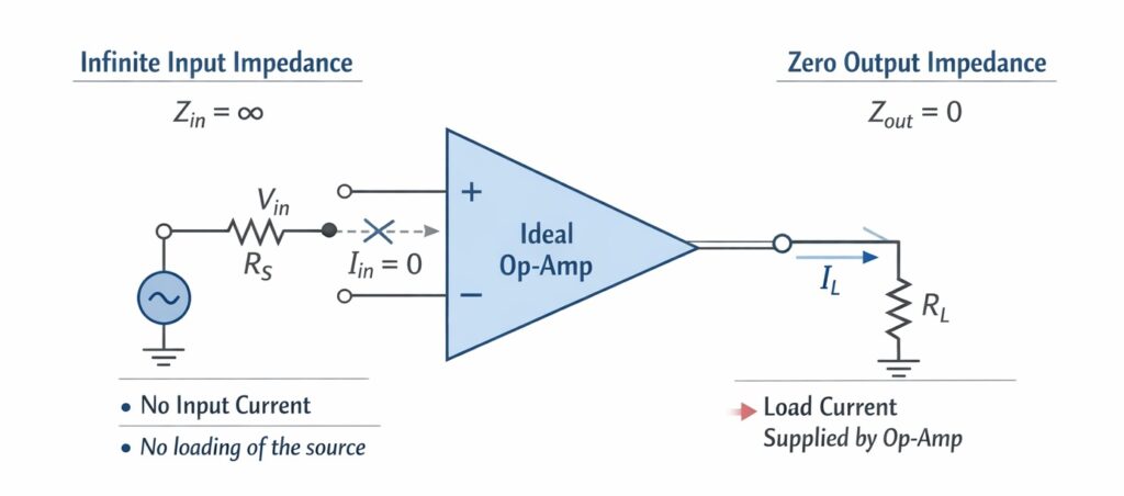
S2: Correct: An ideal operational amplifier has infinite open-loop voltage gain. This very large gain enables accurate amplification and allows the Op-Amp to perform mathematical operations in closed-loop configurations.
\(A_v = \infty\)
S3: Incorrect: An ideal operational amplifier has an infinite slew rate. This means the output voltage can change instantaneously with respect to time. If the slew rate were zero, the output voltage would not change at all, which is practically impossible for an amplifier.
2. An inverting amplifier using the 741C must have a flat response up to 40 kHz. The gain of the amplifier is 10. What maximum peak-to-peak input signal can be applied without distorting the output?
(a) 0.398 V
(b) 3.98 V
(c) 30.98 V
(d) 0.0398 V
Answer: (a) 0.398 V
Solution:
Step 1: Identify the Slew Rate
For a standard 741C operational amplifier, the typical slew rate is
\(SR = 0.5 \, V/\mu s\)
Converting to volts per second:
\(SR = 0.5 \times 10^6 \, V/s\)
Step 2: Determine the Maximum Peak Output Voltage
To avoid distortion due to slew rate limitation, the following condition must be satisfied:
\(SR \ge 2\pi f V_{om}\)
Rearranging the equation:
\(V_{om} = \dfrac{SR}{2\pi f}\)
Substituting the values:
\(V_{om} = \dfrac{0.5 \times 10^6}{2\pi \times 40,000}\)
\(V_{om} \approx \dfrac{500,000}{251,327.4}\)
\(V_{om} \approx 1.989 \, V\) (Peak)
Step 3: Calculate Peak-to-Peak Output Voltage
\(V_{o(p-p)} = 2 \times V_{om}\)
\(V_{o(p-p)} = 2 \times 1.989 \approx 3.978 \, V\)
Step 4: Calculate Maximum Peak-to-Peak Input Voltage
The gain of the amplifier is
\(A = 10\)
Therefore,
\(V_{i(p-p)} = \dfrac{V_{o(p-p)}}{A}\)
\(V_{i(p-p)} = \dfrac{3.978}{10}\)
\(V_{i(p-p)} \approx 0.3978 \, V\)
Rounding to three decimal places,
\(V_{i(p-p)} \approx 0.398 \, V\)
3. Consider the following statements regarding bistable multivibrator:
1. The bistable multivibrator is used as memory elements in shift registers, counters.
2. It is used to generate sine wave by sending regular triggering pulse to the input.
3. It can also be used as a frequency divider.
Which of the above statements is/are correct?
(a) 1 and 3
(b) 3 only
(c) 2 only
(d) 1 and 2
Answer: (a) 1 and 3
Solution:
S1: Correct, a bistable multivibrator has two stable states and remains in one state until an external triggering signal is applied. This property makes it the basic building block of flip-flops. Flip-flops are widely used as memory elements in digital circuits such as shift registers and counters.
Statement 2 is incorrect: Bistable multivibrators are switching circuits that produce digital outputs such as pulses or square waves. They are not used to generate sine waves. Sine wave generation is typically achieved using oscillator circuits such as Wien Bridge oscillators, Hartley oscillators, or RC phase shift oscillators.
![]()
Statement 3 is correct: A bistable multivibrator toggles its state whenever a triggering pulse is applied. Because of this property, the output frequency becomes half of the input triggering frequency. Therefore, it can be used as a frequency divider.
\(f_{out} = \dfrac{f_{in}}{2}\)
4. What is the percentage of resolution of the eight-bit DAC?
(a) 0.0244%
(b) 0.392%
(c) 0.568%
(d) 0.0148%
Answer: (b) 0.392%
Solution:
Step 1: Understand Resolution
The resolution of a Digital-to-Analog Converter (DAC) represents the smallest change in analog output corresponding to a one-bit change in the digital input. For an \(n\)-bit DAC, the total number of output levels is:
\(2^n\)
Step 2: Formula for Percentage Resolution
\(\%\;Resolution = \dfrac{1}{2^n – 1} \times 100\)
Step 3: Substitute the Value
For an 8-bit DAC:
\(n = 8\)
\(\%\;Resolution = \dfrac{1}{2^8 – 1} \times 100\)
\(\%\;Resolution = \dfrac{1}{256 – 1} \times 100\)
\(\%\;Resolution = \dfrac{1}{255} \times 100\)
\(\%\;Resolution \approx 0.39215\%\)
Therefore, the percentage resolution of an 8-bit DAC is approximately 0.392%.
5. What is the value of the capacitance to use in a capacitor filter connected to a full-wave rectifier operating at a standard aircraft power frequency of 400 Hz, if the ripple factor is 10% for a load of 500 \( \Omega \)?
(a) 72.2 µF
(b) 87.6 µF
(c) 25.2 µF
(d) 102.4 µF
Answer: None
Solution:
Step 1: Given Data
Frequency \(f = 400\;Hz\)
Ripple factor \( \gamma = 10\% = 0.1\)
Load resistance \(R_L = 500\;\Omega\)
Step 2: Ripple Factor Formula for Full-Wave Rectifier with Capacitor Filter
\(\gamma = \dfrac{1}{4\sqrt{3}\; f\; C\; R_L}\)
Step 3: Rearranging for Capacitance
\(C = \dfrac{1}{4\sqrt{3}\; f\; \gamma\; R_L}\)
Step 4: Substituting the Values
\(C = \dfrac{1}{4 \times 1.732 \times 400 \times 0.1 \times 500}\)
\(C = \dfrac{1}{138560}\)
\(C \approx 7.217 \times 10^{-6}\;F\)
6. Match the following Lists regarding R-C filter circuit:
| List-I [Component] | List-II [Output voltage (\(V_{out}\))] |
| P. Low-pass filter | 1. \(\dfrac{1}{RC}\int_{0}^{t} V_{in}\,dt\) |
| Q. R-C circuit as integrator | 2. \(V_{in}\dfrac{\omega RC}{\sqrt{1+(\omega RC)^2}}\) |
| R. High-pass filter | 3. \(RC\dfrac{dV_{in}}{dt}\) |
| S. R-C circuit as differentiator | 4. \(V_{in}\dfrac{1}{\sqrt{1+(\omega RC)^2}}\) |
Select the correct answer using the code given below:
(a) P-4, Q-3, R-2, S-1
(b) P-1, Q-3, R-2, S-4
(c) P-2, Q-3, R-4, S-1
(d) P-4, Q-1, R-2, S-3
Answer: (d) P-4, Q-1, R-2, S-3
Solution:
P. Low-pass filter (4): In an RC low-pass filter, the output is taken across the capacitor. The magnitude of the voltage gain is
\(V_{out} = V_{in}\dfrac{1}{\sqrt{1+(\omega RC)^2}}\)
Q. RC circuit as integrator (1): When the time constant \(RC\) is much larger than the input signal period, the circuit behaves as an integrator.
\(V_{out} \approx \dfrac{1}{RC}\int V_{in}\,dt\)
R. High-pass filter (2): In an RC high-pass filter, the output is taken across the resistor. The magnitude of gain is
\(V_{out} = V_{in}\dfrac{\omega RC}{\sqrt{1+(\omega RC)^2}}\)
S. RC circuit as differentiator (3): When the time constant \(RC\) is much smaller than the input signal period, the circuit behaves as a differentiator.
\(V_{out} \approx RC\dfrac{dV_{in}}{dt}\)
7. Match the following Lists:
| List-I (Name of the flag) | List-II (Bit position in flag register) |
| P. Auxiliary carry flag | 1. \(D_0\) |
| Q. Parity flag | 2. \(D_2\) |
| R. Zero flag | 3. \(D_4\) |
| S. Carry flag | 4. \(D_6\) |
Select the correct answer using the code given below:
(a) P-4, Q-3, R-2, S-1
(b) P-3, Q-2, R-4, S-1
(c) P-2, Q-3, R-4, S-1
(d) P-3, Q-2, R-4, S-1
Answer: (b) P-3, Q-2, R-4, S-1
Solution:
In the 8085 microprocessor, the flag register contains five status flags which indicate the result of arithmetic and logical operations.
P. Auxiliary Carry Flag (AC): This flag is set when there is a carry from bit \(D_3\) to \(D_4\). It is located at bit position \(D_4\).
Q. Parity Flag (P): This flag indicates whether the result contains an even or odd number of 1s. It is located at bit position \(D_2\).
R. Zero Flag (Z): This flag becomes 1 if the result of an operation is zero. It is located at bit position \(D_6\).
S. Carry Flag (CY): This flag indicates whether a carry is generated from the most significant bit during arithmetic operations. It is located at bit position \(D_0\).
8. Match the following Lists regarding interfacing the 8155 memory section:
| List-I (Address lines) | List-II (Function used for) |
| P. A11 to A15 | 1. Don’t Care |
| Q. A0 to A7 | 2. Chip Enable |
| R. A8 to A10 | 3. Register Select |
Select the correct answer using the code given below:
(a) P-2, Q-3, R-1
(b) P-1, Q-3, R-2
(c) P-3, Q-2, R-1
(d) P-2, Q-1, R-3
Answer: (a) P-2, Q-3, R-1
Solution:
The 8155 is a multifunction device that includes RAM, I/O ports, and a timer. During interfacing with a microprocessor, different address lines are used for chip selection and register selection.
P. A11 to A15: These higher-order address lines are generally decoded externally to generate the Chip Enable (CE) signal.
Q. A0 to A7: These address lines are used for internal memory addressing and register selection within the 8155.
R. A8 to A10: In many configurations, these lines are not required for internal selection and therefore act as Don’t Care lines.
9. The emission current of a diode is 12.5 mA. What is the rms value of shot noise current for a 10 MHz bandwidth?
(a) 18.2 μA
(b) 1.3 μA
(c) 0.2 μA
(d) 2.7 μA
Answer: (c) 0.2 μA
Solution:
Step 1: Shot Noise Formula
The rms value of shot noise current is given by
\(I_n = \sqrt{2 e I B}\)
Where
\(e = 1.6 \times 10^{-19}\;C\)
\(I = 12.5\,mA = 12.5 \times 10^{-3}\;A\)
\(B = 10\,MHz = 10 \times 10^{6}\;Hz\)
Step 2: Substituting the values
\(I_n = \sqrt{2 \times 1.6 \times 10^{-19} \times 12.5 \times 10^{-3} \times 10 \times 10^{6}}\)
\(I_n = \sqrt{4 \times 10^{-15}}\)
\(I_n = 2 \times 10^{-7.5}\;A\)
\(I_n \approx 0.2\;\mu A\)
10. A transmitter supplies 10 kW power to an aerial, when unmodulated. What is the power radiated when modulated to 30%?
(a) 3 kW
(b) 10.45 kW
(c) 14.8 kW
(d) 4 kW
Answer: (b) 10.45 kW
Solution:
Step 1: Formula for Total Power in AM Wave
\(P_t = P_c\left(1 + \dfrac{m^2}{2}\right)\)
Where
\(P_c =\) Carrier power = \(10\,kW\)
\(m =\) Modulation index = \(30\% = 0.3\)
Step 2: Substituting the values
\(P_t = 10\left(1 + \dfrac{0.3^2}{2}\right)\)
\(P_t = 10\left(1 + \dfrac{0.09}{2}\right)\)
\(P_t = 10(1 + 0.045)\)
\(P_t = 10 \times 1.045\)
\(P_t = 10.45\,kW\)
11. Consider the following statements regarding AM versus FM broadcasting:
1. The process of demodulation is complex in AM broadcasting than that of in FM broadcasting.
2. In FM broadcasting, stereophonic transmission is possible.
3. The AM broadcasting system has poor noise performance.
Which of the above statements is/are correct?
(a) 2 and 3
(b) 3 only
(c) 1 only
(d) 1 and 2
Answer: (a) 2 and 3
Solution:
S1: Incorrect: AM demodulation is relatively simple. A basic envelope detector consisting of a diode and RC circuit can recover the original signal. In contrast, FM demodulation requires more complex circuits such as frequency discriminators, ratio detectors, or phase-locked loop (PLL) demodulators.

S2: Correct: FM broadcasting supports stereophonic transmission. Two audio channels (Left and Right) are transmitted using a multiplexing technique where the sum signal \(L+R\) and difference signal \(L-R\) are transmitted using a subcarrier.
S3: Correct: AM signals are highly susceptible to noise because noise primarily affects the amplitude of signals. Since AM stores information in the amplitude variation of the carrier, noise directly distorts the signal. FM systems provide better noise immunity due to constant amplitude transmission and the capture effect.
12. The signal voltage and noise voltage of a system are 0.923 mV and 0.267 mV respectively. What is the signal-to-noise ratio (SNR) in number?
(a) 3.45
(b) 10.77
(c) 0.29
(d) 11.95
Answer: (d) 11.95
Solution:
Step 1: Formula for Signal-to-Noise Ratio
When SNR is expressed as a power ratio using voltages, it is given by
\(\text{SNR} = \left(\dfrac{V_{signal}}{V_{noise}}\right)^2\)
Step 2: Substitute the given values
\(V_{signal} = 0.923\;mV\)
\(V_{noise} = 0.267\;mV\)
\(\text{SNR} = \left(\dfrac{0.923}{0.267}\right)^2\)
\(\text{SNR} = (3.4569)^2\)
\(\text{SNR} \approx 11.95\)
Therefore, the signal-to-noise ratio is approximately 11.95.
13. Match the following Lists regarding sampling techniques:
| List-I (Sampling technique) | List-II (Principle) |
| P. Natural sampling | 1. It uses sample-hold principle |
| Q. Flat-top sampling | 2. It uses multiplication |
| R. Ideal sampling | 3. It uses multiplication or chopping principle |
Select the correct answer using the code given below:
(a) P-2, Q-3, R-1
(b) P-1, Q-3, R-2
(c) P-3, Q-1, R-2
(d) P-3, Q-2, R-1
Answer: (c) P-3, Q-1, R-2
Solution:
P. Natural sampling (3): In natural sampling, the analog signal is multiplied by a periodic pulse train. The sampled pulses follow the shape of the input signal during the sampling interval, which is also known as the chopping principle.
Q. Flat-top sampling (1): This method uses a sample-and-hold circuit. Each sample is held constant during the sampling interval, producing pulses with flat tops.
R. Ideal sampling (2): Ideal sampling is also called impulse sampling. Mathematically, the signal is multiplied by a train of Dirac delta impulses.
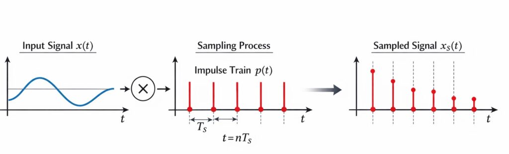
14. The diode falls under which type of system?
(a) Stable only
(b) Unstable only
(c) Either stable or unstable
(d) Neither stable nor unstable
Answer: (a) Stable only
Solution:
In system theory, a system is said to be Bounded-Input Bounded-Output (BIBO) stable if every bounded input produces a bounded output.
A diode is a passive electronic device that cannot generate energy on its own. For any finite input voltage or current applied to a diode, the resulting output voltage or current will also remain finite.
Therefore, a diode satisfies the condition of BIBO stability and is classified as a stable system.
15. Which of the following properties of convolution system exhibits the result of superposition principle for unit impulse response in linear time-invariant systems?
(a) Commutativity only
(b) Distributivity only
(c) Associativity only
(d) Both distributivity and associativity
Answer: (b) Distributivity only
Solution:
The superposition principle states that the response of a linear system to the sum of multiple inputs is equal to the sum of the individual responses produced by each input separately.
In Linear Time-Invariant (LTI) systems, the output is obtained using convolution:
\(y(t) = x(t) * h(t)\)
The distributive property of convolution is
\(x(t) * [h_1(t) + h_2(t)] = x(t)*h_1(t) + x(t)*h_2(t)\)
This property directly represents the superposition principle because the response to a combined impulse response is equal to the sum of the individual responses.
16. The signal space should be divided as
(a) periodic only, whereas the system should be either time scaling or shifting
(b) non-periodic only, whereas the system should be time shifting
(c) either periodic or non-periodic, whereas the system should be either time scaling or shifting
(d) neither periodic nor non-periodic, whereas the system should be time scaling
Answer: (c) either periodic or non-periodic, whereas the system should be either time scaling or shifting
Solution:
In signal processing, signals are broadly classified based on their repetition in time.
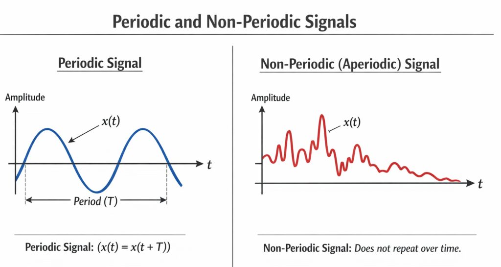
Periodic signals: Signals that repeat after a fixed interval of time. Non-periodic (aperiodic) signals: Signals that do not repeat over time. Thus, the signal space can be divided into periodic and non-periodic signals.
Systems operating on these signals perform operations such as:
Time shifting: \(x(t-t_0)\) which delays or advances the signal.
Time scaling: \(x(at)\) which compresses or expands the time axis.
Therefore, signals may be either periodic or non-periodic, and systems may perform operations such as time scaling or time shifting.
17. Consider a non-recursive filter with the impulse response \(h(n)\) shown in the figure.
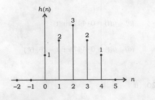
What is the group delay in terms of frequency?
(a) 1
(b) 2
(c) 3
(d) 4
Answer: (b) 2
Solution:
A non-recursive filter corresponds to a Finite Impulse Response (FIR) filter. If the impulse response is symmetric, the filter has linear phase.
The impulse response is
\(h(n) = \{1,2,3,2,1\}\)
The length of the filter is
\(N = 5\)
For a symmetric FIR filter, the group delay is
\(\tau_g = \dfrac{N-1}{2}\)
Substituting \(N = 5\):
\(\tau_g = \dfrac{5-1}{2}\)
\(\tau_g = 2\)
Thus, the group delay of the filter is 2 samples.
18. If \(h(t)=\left[-\dfrac{2}{3}e^{t}+\dfrac{2}{3}e^{-2t}\right]u(-t)+\delta(t)\) , then the function is
(a) causal and stable
(b) non-causal and stable
(c) causal and unstable
(d) non-causal and unstable
Answer: (b) non-causal and stable
Solution:
1. Causality Test
A system is causal if
\(h(t)=0\) for \(t<0\).
Here the impulse response contains the term \(u(-t)\), which is non-zero for negative time. Therefore the system produces output before the input occurs.
Hence, the system is non-causal.
2. Stability Test
An LTI system is BIBO stable if
\(\displaystyle \int_{-\infty}^{\infty}|h(t)|dt<\infty\)
The exponential terms multiplied by \(u(-t)\) decay toward negative infinity and remain bounded, while the impulse term \(\delta(t)\) is also bounded in energy.
Therefore the impulse response is absolutely integrable.
Hence the system is stable.
19. The unit impulse response of an LTI system is
\(h(t)=e^{-t}\sin(2t)u(t)\)
What is the response to \(x(t)=\sin(t)\) using the Laplace transform?
(a) \(y(t)=\sin(2t)\)
(b) \(y(t)=\dfrac{\sin(2t)}{s+1}\)
(c) \(y(t)=0.447\sin(t)\)
(d) \(y(t)=0.447\sin(t-26.6^\circ)\)
Answer: (d) \(y(t)=0.447\sin(t-26.6^\circ)\)
Solution:
Step 1: Determine the transfer function
\(H(s)=\mathcal{L}\{e^{-t}\sin(2t)\}\)
\(H(s)=\dfrac{2}{(s+1)^2+4}\)
\(H(s)=\dfrac{2}{s^2+2s+5}\)
Step 2: Evaluate the frequency response
For the input \(x(t)=\sin(t)\), the frequency is
\(\omega=1\)
Substitute \(s=j\omega=j\)
\(H(j)=\dfrac{2}{(j)^2+2j+5}\)
\(H(j)=\dfrac{2}{-1+2j+5}\)
\(H(j)=\dfrac{2}{4+2j}=\dfrac{1}{2+j}\)
Step 3: Magnitude
\(|H(j)|=\dfrac{1}{\sqrt{2^2+1^2}}=\dfrac{1}{\sqrt{5}}\approx0.447\)
Step 4: Phase
\(\angle H(j)=-\tan^{-1}\left(\dfrac{1}{2}\right)\approx-26.6^\circ\)
Step 5: Output
\(y(t)=0.447\sin(t-26.6^\circ)\)
20. If \(x(n)=\{…,0,0,1,1,1,1,1,1,0,0,…\}\), What is the value of \(y(n)=x(2n)\) ?
(a) \(y(n)=x(2n)+x(n)\)
(b) \(y(n)=u(n)-u(n-7)\)
(c) \(y(n)=u(n)-u(n-4)\)
(d) \(y(n)=x(n)-x(n-7)\)
Answer: (c) \(y(n)=u(n)-u(n-4)\)
Solution:
The sequence \(x(n)\) consists of a block of ones surrounded by zeros.
Down-sampling by a factor of 2 means
\(y(n)=x(2n)\)
This selects every second sample of the original sequence.
Evaluating the samples:
\(y(0)=x(0)=1\)
\(y(1)=x(2)=1\)
\(y(2)=x(4)=1\)
\(y(3)=x(6)=0\)
Thus the resulting sequence is a finite block of ones starting at \(n=0\).
This can be represented using unit step functions as
\(y(n)=u(n)-u(n-4)\)
21. Consider a finite-duration sequence such as \(x(n)=\{1,2,4,8,16\}\). What is the new sequence produced when it revolves 4 units in the circular shift operation?
(a) \(\{4,8,16,1,2\}\)
(b) \(\{2,4,8,16,1\}\)
(c) \(\{1,2,4,8,16\}\)
(d) \(\{16,1,2,4,8\}\)
Answer: (b) \(\{2,4,8,16,1\}\)
Solution:
The original sequence is
\(x(n)=\{1,2,4,8,16\}\)
The sequence length is
\(N=5\)
In a circular shift operation, a right shift of \(k\) samples is defined as
\(x((n-k))_N\)
Here the shift is \(k=4\).
Performing circular right shifts step-by-step:
Original: \(\{1,2,4,8,16\}\)
Shift 1: \(\{16,1,2,4,8\}\)
Shift 2: \(\{8,16,1,2,4\}\)
Shift 3: \(\{4,8,16,1,2\}\)
Shift 4: \(\{2,4,8,16,1\}\)
Thus the new sequence is
\(\{2,4,8,16,1\}\).
22. What is the linear convolution response \(y(5)\) of the sequence \(x(n)=\frac{2}{\sqrt{3}}\sin\left(\frac{\pi n}{3}\right), \quad 0\le n\le5\) and \(h(n)=\{1,2,3,2,1\}\) ?
(a) 0
(b) 9
(c) 14
(d) 28
Answer: (a) 0
Solution:
Step 1: Evaluate \(x(n)\)
\(x(0)=0\)
\(x(1)=1\)
\(x(2)=1\)
\(x(3)=0\)
\(x(4)=-1\)
\(x(5)=-1\)
Thus
\(x(n)=\{0,1,1,0,-1,-1\}\)
Step 2: Convolution formula
\(y(n)=\sum x(k)h(n-k)\)
For \(n=5\)
\(y(5)=x(0)h(5)+x(1)h(4)+x(2)h(3)+x(3)h(2)+x(4)h(1)+x(5)h(0)\)
Since \(h(5)=0\)
\(y(5)=0(0)+1(1)+1(2)+0(3)+(-1)(2)+(-1)(1)\)
\(y(5)=0+1+2+0-2-1=0\)
Therefore
\(y(5)=0\).
23. By using the 3-point DFT of the sequence \(h(n)=a^{-n}\), \(0\le n\le2\), for \(a=1.369\), what is the relationship between the output sequences?
(a) \(H(0)+H(1)+H(2)=4\)
(b) \(H(0)+H(1)=H(2)\)
(c) \(H(1)=H(2)\)
(d) \(H(2)=H^{*}(1)\)
Answer: (d) \(H(2)=H^{*}(1)\)
Solution:
The sequence
\(h(n)=a^{-n}\)
is a real-valued sequence.
For any real sequence, the Discrete Fourier Transform has the conjugate symmetry property
\(H(k)=H^{*}(N-k)\)
For a 3-point DFT, \(N=3\).
Thus
\(H(2)=H^{*}(3-2)\)
\(H(2)=H^{*}(1)\)
This relation holds regardless of the specific value of \(a\).
24. If \(X(s)=\mathcal{L}\{x(t)\}\), determine the initial value \(x(0)\) and final value \(x(\infty)\) for \(X(s)=\dfrac{7s+6}{s(3s+5)}\)
(a) \(\frac{6}{5},\frac{7}{3}\)
(b) \(\frac{7}{3},\frac{7}{3}\)
(c) \(\frac{7}{3},2\)
(d) \(\frac{7}{3},\frac{6}{5}\)
Answer: (d) \(\frac{7}{3},\frac{6}{5}\)
Solution:
Initial Value Theorem
\(x(0)=\lim_{s\to\infty} sX(s)\)
\(x(0)=\lim_{s\to\infty} s\left(\frac{7s+6}{s(3s+5)}\right)\)
\(x(0)=\lim_{s\to\infty}\frac{7s+6}{3s+5}\)
\(x(0)=\frac{7}{3}\)
Final Value Theorem
\(x(\infty)=\lim_{s\to0} sX(s)\)
\(x(\infty)=\lim_{s\to0} s\left(\frac{7s+6}{s(3s+5)}\right)\)
\(x(\infty)=\lim_{s\to0}\frac{7s+6}{3s+5}\)
\(x(\infty)=\frac{6}{5}\)
25. If \(X(s)=\mathcal{L}\{x(t)\}\), find the inverse Laplace transform of \(X(s)=\dfrac{2}{s(s+1)(s+2)^2}\)
(a) \(x(t)=(0.5-2e^{-t}+te^{-2t}+1.5e^{-2t})u(t)\)
(b) \(x(t)=(0.5-2e^{-t}+te^{-2t}+2e^{-2t})u(t)\)
(c) \(x(t)=(0.5-e^{-t}+te^{-2t}+2e^{-2t})u(t)\)
(d) \(x(t)=(1-e^{-t}+te^{-2t})u(t)\)
Answer: (a) \(x(t)=(0.5-2e^{-t}+te^{-2t}+1.5e^{-2t})u(t)\)
Solution:
Step 1: Partial fraction expansion
\(\dfrac{2}{s(s+1)(s+2)^2}=
\dfrac{A}{s}+\dfrac{B}{s+1}+\dfrac{C}{(s+2)^2}+\dfrac{D}{s+2}\)
Step 2: Determine coefficients
\(A=[sX(s)]_{s=0}=\frac{2}{(1)(2^2)}=0.5\)
\(B=[(s+1)X(s)]_{s=-1}=\frac{2}{(-1)(1)^2}=-2\)
\(C=[(s+2)^2X(s)]_{s=-2}=1\)
\(D=1.5\)
Step 3: Inverse Laplace transform
\(\mathcal{L}^{-1}\{\frac{1}{s}\}=1\)
\(\mathcal{L}^{-1}\{\frac{1}{s+1}\}=e^{-t}\)
\(\mathcal{L}^{-1}\{\frac{1}{(s+2)^2}\}=te^{-2t}\)
\(\mathcal{L}^{-1}\{\frac{1}{s+2}\}=e^{-2t}\)
Therefore
\(x(t)=(0.5-2e^{-t}+te^{-2t}+1.5e^{-2t})u(t)\)
26. What is the DC gain (zero frequency) for a system which has a transfer function
\(G(s)=\dfrac{s+2}{(s+1)(s+3)(s+4)}\) ?
(a) \( \dfrac{1}{6} \)
(b) \( \dfrac{2}{3} \)
(c) \( \dfrac{1}{3} \)
(d) \( \dfrac{1}{2} \)
Answer: (a) \( \dfrac{1}{6} \)
Solution:
The DC gain (zero-frequency gain) of a system is obtained by evaluating the transfer function at
\(s=0\).
\(G(0)=\dfrac{0+2}{(0+1)(0+3)(0+4)}\)
\(G(0)=\dfrac{2}{1\times3\times4}\)
\(G(0)=\dfrac{2}{12}\)
\(G(0)=\dfrac{1}{6}\)
Therefore, the DC gain of the system is \(\dfrac{1}{6}\).
27. Match the following Lists:
| List-I (Input Function) | List-II (Use) |
|---|---|
| P. \( \delta(t) \) | 1. Steady-state error |
| Q. \( u(t) \) | 2. Transient response |
| R. \( \sin(\omega t) \) | 3. Transient response and steady-state response |
| S. \( \dfrac{1}{2}t^2 u(t) \) | 4. Transient response modelling steady-state error |
Select the correct answer:
(a) P-1, Q-2, R-3, S-4
(b) P-2, Q-3, R-4, S-1
(c) P-4, Q-2, R-3, S-1
(d) P-2, Q-4, R-3, S-1
Answer: (d) P-2, Q-4, R-3, S-1
Solution:
P. Impulse function \( \delta(t) \)
The impulse input excites all system modes and is mainly used to observe the transient response of the system.
Thus, \(P \rightarrow 2\).
Q. Step input \(u(t)\)
The step input is commonly used to study transient response and steady-state error behaviour of a control system.
Thus, \(Q \rightarrow 4\).
R. Sinusoidal input \( \sin(\omega t) \)
Sinusoidal signals are used in frequency response analysis to determine both transient and steady-state characteristics.
Thus, \(R \rightarrow 3\).
S. Parabolic input \( \dfrac{1}{2}t^2u(t) \)
This input is used to evaluate the steady-state error related to the acceleration error constant.
Thus, \(S \rightarrow 1\).
28. Consider the following steps regarding multiple-node electrical networks:
1. Replace passive elements’ values with their admittance variables
2. Replace all sources and time functions with their Laplace transform
3. Replace transformed voltage sources with transformed current sources
Which of the above steps are correct?
(a) 1 and 2 only
(b) 1 and 3 only
(c) 2 and 3 only
(d) 1, 2 and 3
Answer: (d) 1, 2 and 3
Solution:
For nodal analysis in the s-domain, the following steps are normally followed.
Step 1: Passive components such as resistors, inductors, and capacitors are represented using their admittance forms.
Resistor: \(Y=\dfrac{1}{R}\)
Inductor: \(Y=\dfrac{1}{sL}\)
Capacitor: \(Y=sC\)
Step 2: Time-domain signals and sources are transformed into the Laplace domain.
Step 3: Voltage sources are often converted into equivalent current sources to simplify nodal analysis.
Therefore all three steps are correct.
29. Determine the transfer function \(T(s)=\dfrac{Y(s)}{U(s)}\) for the state-space model
\(\dot{x}=
\begin{bmatrix}
0&1&1\\
0&0&1\\
-1&-2&-3
\end{bmatrix}x+
\begin{bmatrix}
10\\
0\\
0
\end{bmatrix}u\)
\(y=
\begin{bmatrix}
1&0&0
\end{bmatrix}x\)
(a) \(T(s)=\dfrac{10(s^2+3s+2)}{s^3+3s^2+2s+1}\)
(b) \(T(s)=\dfrac{10(s^2+3s+2)}{s^3+3s^2+3s+1}\)
(c) \(T(s)=\dfrac{10(s^2+3s+2)}{s^3+6s^2+5s+1}\)
(d) \(T(s)=\dfrac{10(s^2+3s+2)}{s^3+2s^2+3s+1}\)
Answer: (a) \(T(s)=\dfrac{10(s^2+3s+2)}{s^3+3s^2+2s+1}\)
Solution:
The transfer function from state-space representation is
\(T(s)=C(sI-A)^{-1}B\)
First compute the determinant
\(\det(sI-A)\)
\(
sI-A=
\begin{bmatrix}
s&-1&-1\\
0&s&-1\\
1&2&s+3
\end{bmatrix}
\)
Evaluating the determinant gives
\(s^3+3s^2+2s+1\)
This becomes the denominator of the transfer function.
Multiplying the adjoint matrix with \(B\) and \(C\) gives the numerator
\(10(s^2+3s+2)\)
Thus
\(T(s)=\dfrac{10(s^2+3s+2)}{s^3+3s^2+2s+1}\)
30. Consider the following statements regarding first-order systems:
1. The time constant is the time for \(e^{-\alpha t}\) to decay to 63% of its initial value or the step response to rise to 37% of its final value.
2. Rise time is the time for the waveform to go from 0.1 to 0.9 of its final value.
3. Settling time is the time for the response to remain within 4% of its final value.
Which of the above statements are not correct?
(a) 1 only
(b) 2 only
(c) 3 only
(d) 1 and 3
Answer: (d) 1 and 3
Solution:
Statement 1:
The correct definition is:
For a decaying exponential, the value becomes \(37\%\) of its initial value.
For a rising step response, the output reaches \(63\%\) of its final value.
The statement incorrectly reverses these values. Hence it is incorrect.
Statement 2:
Rise time for a first-order system is generally measured between
\(10\%\) and \(90\%\)
of the final value.
Thus statement 2 is correct.
Statement 3:
Settling time is usually defined using either
\(2\%\) or \(5\%\)
criteria of the final value.
Therefore the 4% definition is not standard and is incorrect.
31. Consider the following statements regarding behavior of second-order underdamped system:
1. The peak time is inversely proportional to the imaginary part of the complex pole.
2. Percent overshoot is a function of only the damping ratio.
3. Settling time is directly proportional to the real part of the complex pole.
Which of the above statements are correct?
(a) 1 and 3 only
(b) 1, 2 and 3
(c) 1 and 2 only
(d) 2 and 3 only
Answer: (c) 1 and 2 only
Solution:
Statement 1:
The peak time of a second-order underdamped system is
\(t_p=\dfrac{\pi}{\omega_d}\)
where \( \omega_d \) is the damped natural frequency, which corresponds to the imaginary part of the complex pole. Therefore peak time is inversely proportional to the imaginary part of the pole.
Thus, Statement 1 is correct.
Statement 2:
The percent overshoot is given by
\(M_p = e^{-\left(\dfrac{\zeta\pi}{\sqrt{1-\zeta^2}}\right)} \times 100\)
This expression depends only on the damping ratio \( \zeta \). Therefore Statement 2 is correct.
Statement 3:
The settling time (for 2% criterion) is approximately
\(t_s=\dfrac{4}{\zeta \omega_n}\)
The real part of the pole is \( -\zeta \omega_n \). Hence settling time is inversely proportional to the real part of the pole, not directly proportional.
Thus Statement 3 is incorrect.
32. For the closed-loop transfer function
\(T(s)=\dfrac{200}{s^4+6s^3+11s^2+6s+200}\)
Determine the system condition based on the number of poles in the left-half plane, right-half plane and the \(j\omega\)-axis.
(a) The system is stable with four poles in the left-half plane
(b) The system is unstable with two right-half plane poles and two left-half plane poles
(c) The system is marginally stable with two poles on the \(j\omega\)-axis
(d) The system is unstable with one right-half plane pole and three left-half plane poles
Answer: (d) The system is unstable with one right-half plane pole and three left-half plane poles
Solution:
The characteristic equation is
\(s^4+6s^3+11s^2+6s+200=0\)
Construct the Routh array.
\(s^4\) : 1 11 200
\(s^3\) : 6 6 0
\(s^2\) : \( \dfrac{6\times11-1\times6}{6}=10 \) 200
\(s^1\) : \( \dfrac{10\times6-6\times200}{10}=-19 \)
\(s^0\) : 200
The first column becomes
1, 6, 10, -19, 200
There is a sign change in the first column indicating the presence of a right-half plane pole. Therefore the system is unstable.
33. Consider the following statements regarding stability for linear time-invariant systems using natural response:
1. A system is marginally stable if the natural response neither decays nor grows but remains constant or oscillates.
2. A system is unstable if the natural response approaches infinity as time approaches zero.
3. A system is unstable if any bounded input yields an unbounded output.
Which of the above statements are not correct?
(a) 1 only
(b) 2 only
(c) 3 only
(d) 2 and 3 only
Answer: (b) 2 only
Solution:
Statement 1:
This describes marginal stability where the natural response neither decays nor grows but remains constant or oscillatory.
Thus Statement 1 is correct.
Statement 2:
A system is unstable if the response grows without bound as \(t \to \infty\), not as \(t \to 0\).
Thus Statement 2 is incorrect.
Statement 3:
This is the definition of BIBO instability: if a bounded input produces an unbounded output.
Thus Statement 3 is correct.
34. What are the values of position constant \(K_p\), velocity constant \(K_v\) and acceleration constant \(K_a\) for a type 0 unity feedback system having
\(G(s)=\dfrac{1000(s+8)}{(s+7)(s+9)}\)
(a) \(K_p=0,\;K_v=0,\;K_a=127\)
(b) \(K_p=0,\;K_v=0,\;K_a=0\)
(c) \(K_p=0,\;K_v=127,\;K_a=127\)
(d) \(K_p=127,\;K_v=0,\;K_a=0\)
Answer: (d) \(K_p=127,\;K_v=0,\;K_a=0\)
Solution
For a unity feedback control system, the static error constants are defined as:
Position constant:
\(K_p = \lim_{s \to 0} G(s)\)
Velocity constant:
\(K_v = \lim_{s \to 0} sG(s)\)
Acceleration constant:
\(K_a = \lim_{s \to 0} s^2G(s)\)
Given Transfer Function
\(G(s)=\dfrac{1000(s+8)}{(s+7)(s+9)}\)
Since the transfer function has no pole at the origin, the system is a Type-0 system.
1. Position Error Constant
\(K_p=\lim_{s \to 0}\dfrac{1000(s+8)}{(s+7)(s+9)}\)
Substituting \(s=0\):
\(K_p=\dfrac{1000(0+8)}{(0+7)(0+9)}\)
\(K_p=\dfrac{8000}{63} \approx 126.98 \approx 127\)
2. Velocity Error Constant
\(K_v=\lim_{s \to 0} sG(s)\)
\(K_v=\lim_{s \to 0} s\dfrac{1000(s+8)}{(s+7)(s+9)}\)
Since \(s \to 0\),
\(K_v = 0\)
3. Acceleration Error Constant
\(K_a=\lim_{s \to 0} s^2G(s)\)
Since \(s^2 \to 0\),
\(K_a = 0\)
Final Result
\(K_p \approx 127,\quad K_v=0,\quad K_a=0\)
Therefore, the correct answer is (d) \(K_p=127,\;K_v=0,\;K_a=0\).
35. Consider the following statements regarding properties of a transfer function:
1. The unit of a transfer function is related to the units of system input and output. A unit is essential.
2. The transfer function can describe only time-invariant linear systems whose parameters remain constant during operation.
3. The transfer function is dependent on the input signal since the characteristics of the system are modified by the input.
Which of the above statements are correct?
(a) 1, 2 and 3
(b) 1 and 3 only
(c) 2 and 3 only
(d) 2 only
Answer: (d) 2 only
Solution:
Statement 1:
The transfer function is defined as
\(G(s)=\dfrac{Y(s)}{X(s)}\)
Although it may carry units depending on input and output variables, the existence of units is not essential to the definition of a transfer function.
Thus Statement 1 is incorrect.
Statement 2:
Transfer functions are defined only for linear time-invariant (LTI) systems.
Thus Statement 2 is correct.
Statement 3:
A transfer function represents the intrinsic characteristics of the system and is independent of the input signal.
Thus Statement 3 is incorrect.
36. Consider the following steps used in performing block diagram reduction to obtain the final transfer function of a system:
Step 1: Combine all serial blocks
Step 2: Close all inner loops
Step 3: Combine all parallel blocks
Step 4: Move summing junctions to the left or right of a block and move take-off (tie) points to the left or right
Select the correct sequence for the above steps.
(a) Step 1, Step 2, Step 3, Step 4
(b) Step 1, Step 3, Step 2, Step 4
(c) Step 3, Step 2, Step 1, Step 4
(d) Step 2, Step 3, Step 1, Step 4
Answer: (b) Step 1, Step 3, Step 2, Step 4
Solution:
In block diagram reduction, the goal is to simplify the system step by step.
Step 1: First combine cascading (series) blocks. If two blocks are in series with transfer functions \(G_1(s)\) and \(G_2(s)\), the equivalent block becomes
\(G(s) = G_1(s)G_2(s)\)
Step 3: Next combine parallel blocks. If blocks are in parallel, the equivalent transfer function becomes
\(G(s) = G_1(s) + G_2(s)\)
Step 2: After simplifying series and parallel connections, eliminate inner feedback loops using
\(G_{eq}(s)=\dfrac{G(s)}{1+G(s)H(s)}\)
Step 4: If required, move summing junctions and take-off points to simplify the diagram further.
Therefore, the correct sequence is
Step 1 → Step 3 → Step 2 → Step 4
37. Consider the following statements regarding representation of block diagrams through signal flow diagrams:
1. The signal at a node is equal to the sum of all signals transmitted to the node. Sometimes the transmittance may be positive.
2. The transmittances are simply related to the transfer functions.
3. The transmittances connected to the input/output nodes are both unity and merely help to make the diagram clearer.
Which of the above statements is/are correct?
(a) 2 and 3
(b) 1 and 3
(c) 1 and 2
(d) 1 only
Answer: (c) 1 and 2
Solution:
Statement 1:
In a signal flow graph, each node represents a variable. The value at a node is equal to the algebraic sum of all incoming signals multiplied by their branch transmittances.
Therefore Statement 1 is correct.
Statement 2:
The branch transmittance represents the gain or transfer function between two nodes. Hence transmittances are directly related to transfer functions.
Therefore Statement 2 is correct.
Statement 3:
The branches connected to input or output nodes do not necessarily have unity transmittance. Their values depend on the system model.
Therefore Statement 3 is incorrect.
38. Consider the following statements regarding Nyquist stability criterion:
1. The Nyquist stability criterion is a geometric and graphical method in the frequency domain.
2. It uses the open-loop Nyquist plot to determine the stability of the closed-loop system.
3. Instead of solving characteristic roots, the Nyquist criterion determines stability using the open-loop frequency response.
Which of the above statements are correct?
(a) 1, 2 and 3
(b) 1 and 3 only
(c) 1 and 2 only
(d) 2 and 3 only
Answer: (a) 1, 2 and 3
Solution:
Statement 1:
The Nyquist stability criterion is a graphical technique used in the frequency domain. It examines the Nyquist plot of the open-loop transfer function.
Thus Statement 1 is correct.
Statement 2:
The stability of a closed-loop system is determined from the open-loop transfer function \(G(s)H(s)\) using the Nyquist plot.
Thus Statement 2 is correct.
Statement 3:
The Nyquist criterion avoids directly solving the characteristic equation. Instead, it evaluates stability using frequency response plots.
Thus Statement 3 is correct.
39. A transformer on no-load has a core loss of 50 W, draws a current of 2 A (rms) and has an induced emf of 230 V (rms). What is the core loss current?
(a) 0.216 A
(b) 1.988 A
(c) 2.328 A
(d) 0.456 A
Answer: (a) 0.216 A
Solution:
At no-load, the input current consists of two components:
1. Core loss current \(I_c\)
2. Magnetizing current \(I_m\)
The core loss is related to the core loss current by
\(P_i = E I_c\)
where
\(P_i\) = core loss
\(E\) = induced emf
Substitute the given values:
\(I_c = \dfrac{P_i}{E}\)
\(I_c = \dfrac{50}{230}\)
\(I_c \approx 0.217 \text{ A}\)
The closest value is 0.216 A
40. A 500 kVA transformer has an efficiency of 95% at full load and also at 60% of full load, both at unity power factor. Determine the iron loss and copper loss.
(a) \(P_i=12.42\text{ kW},\; P_c=18.52\text{ kW}\)
(b) \(P_i=2.45\text{ kW},\; P_c=8.35\text{ kW}\)
(c) \(P_i=8.43\text{ kW},\; P_c=13.25\text{ kW}\)
(d) \(P_i=9.87\text{ kW},\; P_c=16.45\text{ kW}\)
Answer: (d) \(P_i=9.87\text{ kW},\; P_c=16.45\text{ kW}\)
Solution:
Step 1: Full load condition
Output power
\(P_{out}=500 \times 1 = 500 \text{ kW}\)
Efficiency
\(\eta=\dfrac{Output}{Input}=0.95\)
Input power
\(Input=\dfrac{500}{0.95}=526.32 \text{ kW}\)
Total losses
\(P_i + P_c = 526.32 – 500 = 26.32 \text{ kW}\)
Step 2: At 60% load
Output power
\(P_{out}=500 \times 0.6 = 300 \text{ kW}\)
Input power
\(Input=\dfrac{300}{0.95}=315.79 \text{ kW}\)
Total losses
\(P_i + (0.6)^2 P_c = 315.79 – 300\)
\(P_i + 0.36P_c = 15.79 \text{ kW}\)
Step 3: Solve equations
\(P_i + P_c = 26.32\)
\(P_i + 0.36P_c = 15.79\)
Subtracting
\(0.64P_c = 10.53\)
\(P_c \approx 16.45 \text{ kW}\)
\(P_i = 26.32 – 16.45\)
\(P_i \approx 9.87 \text{ kW}\)
Thus
\(P_i = 9.87 \text{ kW},\quad P_c = 16.45 \text{ kW}\)
41. Consider the following statements regarding three-phase transformer connections:
1. Delta/Delta is economical for small HV transformers.
2. Star/Star suits large LV transformers.
3. Star/Delta is the most commonly used connection for power systems.
Which of the above statements is/are correct?
(a) 2 and 3
(b) 3 only
(c) 1 only
(d) 1 and 2
Answer: (b) 3 only
Solution:
Statement 1:
Delta–Delta connection is generally used for low-voltage and high-current applications. It is not economical for high-voltage transformers because insulation requirements become large.
Thus Statement 1 is incorrect.
Statement 2:
Star–Star connection is normally preferred for high-voltage transformers because the phase voltage becomes
\(V_{ph} = \dfrac{V_L}{\sqrt{3}}\)
This reduces insulation requirement. Hence it is suitable for high-voltage applications rather than large LV transformers.
Thus Statement 2 is incorrect.
Statement 3:
Star–Delta and Delta–Star connections are widely used in power systems. Star–Delta is commonly used in substations for step-down transformers.
Thus Statement 3 is correct.
42. A 240 V / 120 V, 12 kVA transformer has full-load unity power factor efficiency of 96.2%. It is connected as an auto-transformer to feed a load at 360 V. What is the auto-transformer rating?
(a) 36 kVA
(b) 18 kVA
(c) 54 kVA
(d) 34.63 kVA
Answer: (a)
Explanation: When a two-winding transformer is reconnected as an auto-transformer, a part of the power is transferred conductively (directly) and the rest inductively. This increases the kVA rating without changing the current rating of the windings.
Given:
- Two-winding rating = 12 kVA
- Voltages = 240 V and 120 V
- Auto-transformer output voltage = 360 V (series additive connection)
Auto-transformer kVA rating is given by:
\( S_{auto} = S_{tw} \times \dfrac{V_{total}}{V_{series}} \)
\( = 12 \times \dfrac{360}{120} = 12 \times 3 = 36 \text{ kVA} \)
Thus, the auto-transformer rating is 36 kVA.
43. The magnetic flux density on the surface of an iron face is 1.6 T, which is a typical saturation level value for ferromagnetic material. What is the force density on the iron face?
(a) 1.6 × 10⁶ N/m²
(b) 1.02 × 10⁶ N/m²
(c) 1.02 × 10⁷ N/m²
(d) 1.6 × 10⁷ N/m²
Answer: (b)
Explanation:
The magnetic force density (pressure) acting on a surface is given by:
\( F = \dfrac{B^2}{2\mu_0} \)
where,
\( B = 1.6 \, \text{T} \)
\( \mu_0 = 4\pi \times 10^{-7} \, \text{H/m} \)
Substituting the values:
\( F = \dfrac{(1.6)^2}{2 \times 4\pi \times 10^{-7}} \)
\( = \dfrac{2.56}{8\pi \times 10^{-7}} \approx 1.02 \times 10^6 \, \text{N/m}^2 \)
Thus, the force density on the iron face is approximately 1.02 × 10⁶ N/m².
44. For a 6-pole DC armature with 16 slots having two coil sides per slot and single-turn coils, what is the commutator pitch (Yc) for a wave winding?
(a) 8 segments
(b) 9 segments
(c) 6 segments
(d) 5 segments
Answer: (c)
Explanation:
For a DC machine with wave winding, the commutator pitch is given by:
\( Y_c = \dfrac{C \pm 1}{P/2} \)
where,
\( C = 16 \) (number of coils)
\( P = 6 \) (number of poles)
Using the additive (+) sign:
\( Y_c = \dfrac{16 + 1}{3} = \dfrac{17}{3} \approx 6 \)
Hence, the commutator pitch is approximately 6 segments.
45. Consider the following statements regarding speed control of DC motors:
1. In field control method, speeds higher than the rated speed cannot be obtained.
2. For motors requiring a wide range of speed control, field control method leads to unstable operating conditions or poor commutation.
3. Field control method is not suited to applications needing speed reversal.
(a) 2 and 3
(b) 3 only
(c) 1 only
(d) 1 and 2
Answer: (a)
Explanation:
- Statement 1: Incorrect. Field control is used to obtain speeds higher than rated speed by weakening the flux.
- Statement 2: Correct. Wide-range field weakening can lead to poor commutation and instability.
- Statement 3: Correct. Field control is not suitable for speed reversal; armature control is preferred.
Therefore, statements 2 and 3 are correct.
46. Which one of the following is not the remedy for reducing cross-magnetizing effect of the armature reaction?
(a) Introducing saturation in the teeth and pole shoe
(b) By chamfering the pole shoes which increases the air gap at the pole tips
(c) By making the field circuit resistance more than the critical value
(d) Compensating the armature reaction mmf by a compensating winding located in the pole shoes
Answer: (c)
Explanation: The cross-magnetizing effect of armature reaction can be reduced by:
- Introducing saturation in pole shoes and teeth
- Chamfering pole shoes to modify flux distribution
- Using compensating windings to counteract armature mmf
However, increasing the field circuit resistance beyond the critical value is related to voltage build-up in generators and does not reduce armature reaction.
Hence, option (c) is correct.
47. The total iron losses in the armature of a DC machine running at 875 rpm are 1100 W. What is the approximate braking torque due to iron losses?
(a) 8 N-m
(b) 16.42 N-m
(c) 8.85 N-m
(d) 12 N-m
Answer: (d)
Explanation:
Braking torque due to iron losses is given by:
\( T = \dfrac{P}{\omega} \)
where,
\( P = 1100 \, \text{W} \)
\( \omega = \dfrac{2\pi N}{60} = \dfrac{2\pi \times 875}{60} \)
\( \omega \approx 91.63 \, \text{rad/s} \)
\( T = \dfrac{1100}{91.63} \approx 12 \, \text{N-m} \)
Hence, the braking torque is approximately 12 N-m.
48. A 0.5 hp, 6-pole induction motor is excited by a 3-phase, 60 Hz source. If the full-load speed is 1140 rpm, what is the percentage of slip?
(a) 6%
(b) 12%
(c) 5%
(d) 3%
Answer: (c)
Explanation:
Synchronous speed is given by:
\( N_s = \dfrac{120 f}{P} = \dfrac{120 \times 60}{6} = 1200 \, \text{rpm} \)
Slip is:
\( s = \dfrac{N_s – N}{N_s} = \dfrac{1200 – 1140}{1200} = \dfrac{60}{1200} = 0.05 \)
\( s = 5\% \)
Hence, the percentage slip is 5%.
49. A \(50\ \text{Hz}\) induction motor wound for pole-amplitude modulation has \(20\) initial poles and the modulating function has \(8\) poles. At what two speeds will the motor run?
(a) \(300\ \text{rpm}\) and \(214.286\ \text{rpm}\)
(b) \(400\ \text{rpm}\) and \(318.524\ \text{rpm}\)
(c) \(150\ \text{rpm}\) and \(414.495\ \text{rpm}\)
(d) \(450\ \text{rpm}\) and \(115.359\ \text{rpm}\)
Ans. (a)
Explanation: In pole-amplitude modulation (PAM), the resulting number of poles is given by:
\( P = P_1 \pm P_m \)
where
- \( P_1 = 20 \) (initial poles)
- \( P_m = 8 \) (modulating poles)
Hence, the possible pole combinations are:
\( P = 20 + 8 = 28 \), and \( P = 20 – 8 = 12 \)
The synchronous speed is given by:
\( N_s = \dfrac{120 f}{P} \)
- For \( P = 20 \):
\( N_s = \dfrac{120 \times 50}{20} = 300\ \text{rpm} \) - For \( P = 28 \):
\( N_s = \dfrac{120 \times 50}{28} = 214.286\ \text{rpm} \)
Therefore, the motor runs at \(300\ \text{rpm}\) and \(214.286\ \text{rpm}\).
50. A 3-phase synchronous generator produces an open-circuit line voltage of \(6928\ \text{V}\), when the DC exciting current is \(50\ \text{A}\). The AC terminals are then short-circuited and the three line currents are found to be \(800\ \text{A}\). What is the synchronous reactance per phase?
(a) \(138.5\ \Omega\)
(b) \(8.6\ \Omega\)
(c) \(80\ \Omega\)
(d) \(5\ \Omega\)
Ans. (d) \(5\ \Omega\)
Explanation:
The synchronous reactance per phase is given by:
\( X_s = \dfrac{E_{\text{ph}}}{I_{\text{sc}}} \)
where
- \( E_{\text{ph}} \) = open-circuit phase voltage
- \( I_{\text{sc}} \) = short-circuit current
Convert line voltage to phase voltage:
\( E_{\text{ph}} = \dfrac{6928}{\sqrt{3}} = 4000\ \text{V} \)
Given short-circuit current:
\( I_{\text{sc}} = 800\ \text{A} \)
Therefore,
\( X_s = \dfrac{4000}{800} = 5\ \Omega \)
Hence, the synchronous reactance per phase is \(5\ \Omega\).
51. Consider the following advantages of hydrogen cooling of alternators in steam power generation:
1. Less noise due to the lower density of hydrogen.
2. Ventilation losses (fan power absorbed) are higher by 10%.
3. The heat transfer is more than that of air.
Which of the above advantages is/are correct?
(a) 2 and 3
(b) 2 only
(c) 1 only
(d) 1 and 3
Answer: (d) 1 and 3
Solution:
S1: Hydrogen has a density nearly 1/14th that of air. Because of the lower density, windage loss in the rotor is reduced. This also results in quieter operation and therefore less noise. Hence Statement 1 is correct.
S2: Ventilation or windage losses depend on the density of the cooling medium. Since hydrogen is much lighter than air, the ventilation losses are actually lower, not higher. Therefore Statement 2 is incorrect.
S3: Hydrogen has a much higher thermal conductivity compared to air, which improves heat transfer and cooling efficiency in large alternators. Hence Statement 3 is correct.
Therefore, the correct answer is 1 and 3.
52. Match List I with List II regarding Surge Impedance Loading (SIL) of AC transmission lines
| List I (Conductor configuration and line voltage) |
List II (SIL in MW) |
|---|---|
| (P) Quad Bersimis – 400 kV | (1) 647 |
| (Q) Twin Moose – 400 kV | (2) 605 |
| (R) Quad Zebra – 400 kV | (3) 691 |
| (S) Triple Snowbird – 400 kV | (4) 515 |
Select the correct answer using the code given below:
(a) 3 4 1 2
(b) 2 1 4 3
(c) 1 4 2 3
(d) 4 3 2 1
Answer: (a)
Solution:
Surge Impedance Loading (SIL) represents the natural loading of a transmission line at which the reactive power generated by the line capacitance equals the reactive power absorbed by the line inductance.
The SIL of a transmission line is given by
\( SIL = \dfrac{V^2}{Z_c} \)
where
\(V\) = line voltage
\(Z_c\) = surge impedance of the transmission line
The value of surge impedance depends strongly on the conductor configuration. Increasing the number of sub-conductors in a bundle reduces inductive reactance and increases capacitance. This reduces surge impedance and increases the surge impedance loading.
Correct Matching:
P. Quad Bersimis – 400 kV → 691 MW
Q. Twin Moose – 400 kV → 515 MW
R. Quad Zebra – 400 kV → 647 MW
S. Triple Snowbird – 400 kV → 605 MW
53. If \(d\) is the distance between the conductors and \(e\) is Euler’s number, determine the conductor radius \(r\) at which the maximum critical disruptive voltage occurs.
(a) \(d \times e\)
(b) \(\dfrac{d}{1-e}\)
(c) \(\dfrac{d}{e}\)
(d) \(\dfrac{d}{1+e}\)
Answer: (c) \(\dfrac{d}{e}\)
Solution:
The disruptive critical voltage for corona formation in a transmission line is given by
\(V_c = m_0 g r \delta \ln\!\left(\dfrac{d}{r}\right)\)
where
\(m_0\) = surface irregularity factor
\(g\) = breakdown strength of air
\(\delta\) = air density factor
\(d\) = distance between conductors
\(r\) = radius of conductor
To obtain the maximum disruptive voltage, differentiate the expression with respect to \(r\) and equate it to zero.
\(\dfrac{d}{dr}\left[r \ln\left(\dfrac{d}{r}\right)\right] = 0\)
Simplifying gives
\(\ln\left(\dfrac{d}{r}\right) – 1 = 0\)
\(\ln\left(\dfrac{d}{r}\right) = 1\)
Taking exponential on both sides:
\(\dfrac{d}{r} = e\)
Therefore
\(r = \dfrac{d}{e}\)
Hence the conductor radius for maximum disruptive voltage is
\(r = \dfrac{d}{e}\)
54. Match List I with List II regarding cable conductors
| List I (Property) | List II (Value) |
|---|---|
| (P) Specific gravity of copper | (1) 15 kg/mm² |
| (Q) Ultimate tensile strength of copper | (2) 8.890 |
| (R) Specific gravity of aluminium | (3) 40 kg/mm² |
| (S) Ultimate tensile strength of aluminium | (4) 2.71 |
Select the correct answer using the code given below:
(a) 3 4 1 2
(b) 2 3 4 1
(c) 1 3 4 2
(d) 4 1 2 3
Answer: (b)
Explanation:
Copper is significantly denser and possesses higher mechanical strength than aluminium.
- Specific gravity of copper ≈ 8.890.
- Ultimate tensile strength of copper ≈ 40 kg/mm².
- Specific gravity of aluminium ≈ 2.71.
- Ultimate tensile strength of aluminium ≈ 15 kg/mm².
Therefore, the correct matching is:
P → 2, Q → 3, R → 4, S → 1
Hence the correct code is 2 3 4 1.
55. Match List I with List II regarding percentage distribution of faults in various elements of a power system
| List I (Element) | List II (% of total fault) |
|---|---|
| (P) Overhead lines | (1) 10 |
| (Q) Underground cables | (2) 50 |
| (R) Transformers | (3) 7 |
| (S) Generators | (4) 9 |
Select the correct answer using the code given below:
| Option | P | Q | R | S |
|---|---|---|---|---|
| (a) | 3 | 4 | 1 | 2 |
| (b) | 2 | 1 | 4 | 3 |
| (c) | 2 | 4 | 1 | 3 |
| (d) | 2 | 3 | 4 | 1 |
Answer: (b)
Explanation:
The percentage distribution of faults in different elements of a power system varies due to exposure, insulation conditions, and operating stresses.
- Overhead lines experience the highest number of faults due to exposure to weather conditions such as lightning, wind, and tree contact. Their fault contribution is about 50%.
- Underground cables contribute around 10% of the total faults.
- Transformers account for approximately 9% of faults.
- Generators contribute about 7% of the total faults.
Correct Matching:
P → 2 (50)
Q → 1 (10)
R → 4 (9)
S → 3 (7)
Hence, the correct code is 2 1 4 3.
56. For a 735 kV transmission line with a fault current of 4 kA, determine the arc resistance. Assume no resistance in the ground return path.
(a) 4 Ω
(b) 8 Ω
(c) 183.75 Ω
(d) 0.183 Ω
Answer: (c) 183.75 Ω
Solution:
The arc resistance during a fault can be approximated by using Ohm’s law.
\(R = \dfrac{V}{I}\)
where
\(V\) = line voltage
\(I\) = fault current
Given
Line voltage \(V = 735 \text{ kV}\)
Fault current \(I = 4 \text{ kA}\)
Substituting the values:
\(R = \dfrac{735 \times 10^3}{4 \times 10^3}\)
\(R = \dfrac{735}{4}\)
\(R = 183.75 \; \Omega\)
Thus the arc resistance is
183.75 Ω
57. Consider the following statements regarding static relays compared with electromechanical relays:
1. In static relays, frequent operations cause deterioration.
2. In static relays, there is quick resetting and absence of overshoot.
3. Static relays are sensitive to voltage transients.
Which of the above statements is/are correct?
(a) 2 and 3
(b) 2 only
(c) 1 only
(d) 1 and 3
Answer: (a) 2 and 3
Solution:
S1: Static relays are electronic devices and do not contain moving mechanical parts. Therefore, frequent operations do not cause mechanical wear or deterioration. Hence Statement 1 is incorrect.
S2: Since static relays use semiconductor components and electronic circuits, they have very fast response and quick resetting. They also do not suffer from mechanical overshoot. Thus Statement 2 is correct.
S3: Static relays are sensitive to voltage spikes and transients because semiconductor devices can be affected by sudden over-voltages. Thus Statement 3 is correct.
58. What is the maximum value of restriking voltage across the contacts of a circuit breaker in a 132 kV system?
(a) 107.78 kV
(b) 215.56 kV
(c) 93.35 kV
(d) 186.64 kV
Answer: (b) 215.56 kV
Solution:
This value is determined by the peak phase-to-neutral voltage of the system. In a standard three-phase power system, the “132 kV” rating refers to the Line-to-Line RMS voltage (\(V_{LL(RMS)}\)).
Calculation Steps
- Calculate the Phase RMS Voltage (\(V_{Ph(RMS)}\)):
\[
V_{Ph(RMS)} = \frac{V_{LL(RMS)}}{\sqrt{3}} = \frac{132 \text{ kV}}{\sqrt{3}} \approx 76.21 \text{ kV}
\] - Calculate the Peak Phase Voltage (\(V_m\)):
\[
V_m = V_{Ph(RMS)} \times \sqrt{2} = 76.21 \text{ kV} \times \sqrt{2} \approx 107.78 \text{ kV}
\] - Determine Maximum Restriking Voltage (\(V_{tr(max)}\)):The restriking voltage expression is:
\[
v_c(t) = V_m (1 – \cos \omega_n t)
\]The maximum value occurs when the cosine term is \(-1\):
\[
V_{tr(max)} = 2 \times V_m = 2 \times 107.78 \text{ kV} \approx \mathbf{215.56 \text{ kV}}
\]
59. Consider the following statements regarding radial distribution systems:
1. Distributor far away from the substation is highly loaded.
2. Severe voltage variation to the consumers nearest to the substation is due to load variations.
3. Consumers are dependent on a single feeder and a single distributor, and a fault on either of them causes interruption of supply to all the consumers away from the fault.
Which of the above statements is/are correct?
(a) 2 and 3
(b) 3 only
(c) 1 only
(d) 1 and 3
Answer: (b) 3 only
Solution:
S1: In a radial distribution system, the distributor is most heavily loaded near the feeding point (substation), not at the far end. Thus Statement 1 is incorrect.
S2: Voltage variations are usually more severe at consumers located farthest from the substation because of the voltage drop along the distribution line. Thus Statement 2 is incorrect.
S3: In a radial system, all consumers are supplied through a single path. Therefore a fault in the feeder or distributor interrupts supply to all consumers beyond the fault location. Thus Statement 3 is correct.
60. Match the following Lists regarding bus classifications:
| List–I (Bus Type) | List–II (Quantities to be obtained) | |
|---|---|---|
| P. Generator bus | 1. Real power, reactive power | |
| Q. Load bus | 2. Reactive power, phase angle | |
| R. Slack bus | 3. Voltage magnitude, phase angle |
Select the correct answer using the code given below.
(a) 2 3 1
(b) 3 2 1
(c) 2 1 3
(d) 1 3 2
Answer: (a) 2 3 1
Solution:
In power flow studies, buses are classified based on the quantities specified and the quantities to be determined.
Generator bus (PV bus):
Voltage magnitude and real power are specified. The unknown quantities are reactive power and phase angle.
Thus P → 2.
Load bus (PQ bus):
Real and reactive powers are specified. The unknown quantities are voltage magnitude and phase angle.
Thus Q → 3.
Slack bus:
Voltage magnitude and phase angle are specified. The unknown quantities are real and reactive power.
Thus R → 1.
61. Consider the following statements with respect to the change in torque angle whenever a disturbance occurs:
1. There is no change in torque angle when the speed of the rotor is the synchronous speed.
2. The angle decreases in case of a motor, if \( P_s > P_e \), i.e., the mechanical output is more than the electrical input and the speed goes down.
3. The angle increases, if the speed is more than the synchronous speed.
Which of the above statements is/are correct?
(a) 2 and 3
(b) 3 only
(c) 1 only
(d) 1 and 3
Ans. (c) 1 only
Explanation: The torque angle remains constant only when the rotor runs at synchronous speed. Any deviation in speed due to disturbance changes the torque angle. Hence, only statement 1 is correct.
62. Which one of the following is not a feature of an ideal control system for an HVDC converter?
(a) Control should require less reactive power.
(b) The DC current is constant (ripple-free).
(c) Under steady-state conditions, the valve must be fired symmetrically.
(d) Continuous operating range from full rectification to full inversion.
Ans. (c)
Explanation: Ideal HVDC control aims at stable, efficient operation with minimum reactive power and smooth DC current. Symmetrical firing is not a necessary or defining feature.
63. Consider the following statements regarding Static Synchronous Compensator (STATCOM):
1. It is insensitive to transmission system harmonics.
2. It has difficulty operating with a very weak AC system.
3. It can be used for a small amount of energy storage.
Which of the above statements is/are correct?
(a) 2 and 3
(b) 3 only
(c) 1 only
(d) 1 and 3
Ans. (d) 1 and 3
Explanation: STATCOM is largely insensitive to harmonics and can provide limited energy storage through its DC capacitor. It performs well even in weak systems, so statement 2 is incorrect.
64. A diode circuit consists of a diode in series with switch \( S_1 \), resistance \( R = 44\ \Omega \) and capacitance \( C = 0.1\ \mu F \). The capacitor has an initial voltage \( V_c(0) = 220\ V \). If switch \( S_1 \) is closed at \( t = 0 \), what is the energy dissipated in the resistor \( R \)?
(a) \(3.86\ \text{mJ}\)
(b) \(5\ \text{mJ}\)
(c) \(139.64\ \text{mJ}\)
(d) \(2.42\ \text{mJ}\)
Ans. (d) \(2.42\ \text{mJ}\)
Explanation: Energy dissipated equals initial energy stored in the capacitor: \( E = \dfrac{1}{2} C V^2 = \dfrac{1}{2} \times 0.1 \times 10^{-6} \times (220)^2 = 2.42\ \text{mJ} \)
65. Which of the following is not a limitation of MOSFET?
(a) High on-state voltage drop
(b) Unipolar device
(c) Slower switching speed
(d) Lower off-state voltage capability
Ans. (b)
Explanation: MOSFET is a unipolar device, which is an advantage (fast switching), not a limitation. Other options represent actual limitations.